Lecture 12

Network Psychometrics

Jihong Zhang

Educational Statistics and Research Methods

Today’s Objectives

1. Understand what is network psychometrics and

2. Understand the relationship between psychometric/psychological network with factor analysis

3. Understand how network model can be applied into real scenarios

Background

Network Analysis

Network analysis is a broad area. It has many names in varied fields:

1. Graphical Models (Computer Science, Machine Learning)
2. Bayesian Network (Computer Science, Educational Measurement)
3. Social Network (Sociology)
4. Psychological/Psychometric Network (Psychopathology, Psychology)
5. Structural Equation Model, Path Analysis (Psychology, Education)

1 and 2 focus on the probabilistic relationships and further casual relationships among variables. 3 and 4 focuses on network structure and node importance. 5 focus on the regression coefficients of structural and measurement mdoel.

All 5 analysis methods have a network-shaped diagram. Graphical modeling is a more “general” term that can comprise of the other network models.

Examples of varied networks

Figure 1: Bayesian Network (Briganti et al., 2023)

Figure 2: Facebook friendship network in a single undergraduate dorm (Lewis et al., 2008)

Figure 3: Factor Analysis and Psychological Network (Borsboom et al., 2021)

Research Aims

1. Bayesian Network (BN) aims to derive the casual relations between variables
2. Social Network aims to examine the network structure (community, density or centrality) of individuals
3. Factor Analysis aims to identify latent variables
4. Psychological Network aims to examines the associations among observed variables (topological structures) and their positions in the network.

Network Psychometrics

1. Network psychometrics is a novel area that allows representing complex phenomena of measured constructs in terms of a set of elements that interact with each other.
2. It is inspired by the so-called mutualism model and research in ecosystem modeling (Kan, Maas, and Levine 2019).
   • A mutualism model proposes that basic cognitive abilities directly and positively interact during development.
3. Psychometric network arises as dynamics or reciprocal causation among variables are getting more attentions.
4. For example, individual differences in depression could arise from, and could be maintained by, vicious cycles of mutual relationships among symptoms.
5. A depression symptom such as insomnia can cause another symptom, such as fatigue, which in turn can determine concentration problems and worrying, which can result in more insomnia and so on.

Comparison to factor analysis

Factor analysis (common factor model) assumes the associations between observed features can be explained by one or more common factors.

• For example, higher “depression” level leads to increased frequency of depressive behaviors

Psychometric network, however, assumes the associations between observed features ARE the reason of the development of depression. Or “depression” is the network itself.

• unavoidable cycle of “fatigue -> worrying -> insomnia -> fatigue” will leads to higher “depression”

Utility of Psychometric Network

1. Explain the pathways of certain psychological phenomenon
2. Identify the most important problem that needed to be intervene in the treatment procedure
3. Examine group differences in interactions among observed features
4. Examine density of network: more dense network indicates more dynamic of certain problems
5. Examine clusters/communities of observed features: some symptoms are more likely to concur than other symptoms

Terminology I - Overall procedure

1. Network structure estimation: the application of statistical models to assess the structure of pairwise (conditional) associations in multivariate data.
2. Network description: characterization of the global topology and the position of individual nodes in that topology.
3. Psychometric network analysis: the analysis of multivariate psychometric data using network structure estimation and network description.

Terminology II - Network description

1. Node: psychometric variables that are selected in the network
   • such as responses to questionnaire items, symptom ratings, and cognitive test scores, background variables such as age and gender, experimental interventions.
2. Edge (conditional association): associations between variables taking into account other variables that may explain the association
3. Edge weight: parameter estimates that represent the strength of conditional association between nodes
4. Node centrality: the relative importance of a node in the context of other nodes, that can be calculated using different statistics

Terminology III - Network structure estimation

1. Node selection: the choice of which variables will function as nodes in the network model.
2. Network stability analysis: the assessment of estimation precision and robustness to sampling error of psychometric networks.
3. Pairwise Markov random field (PMRF): an undirected network that represents variables as nodes and conditional associations as edges, in which unconnected nodes are conditionally independent.

Exploratory Nature

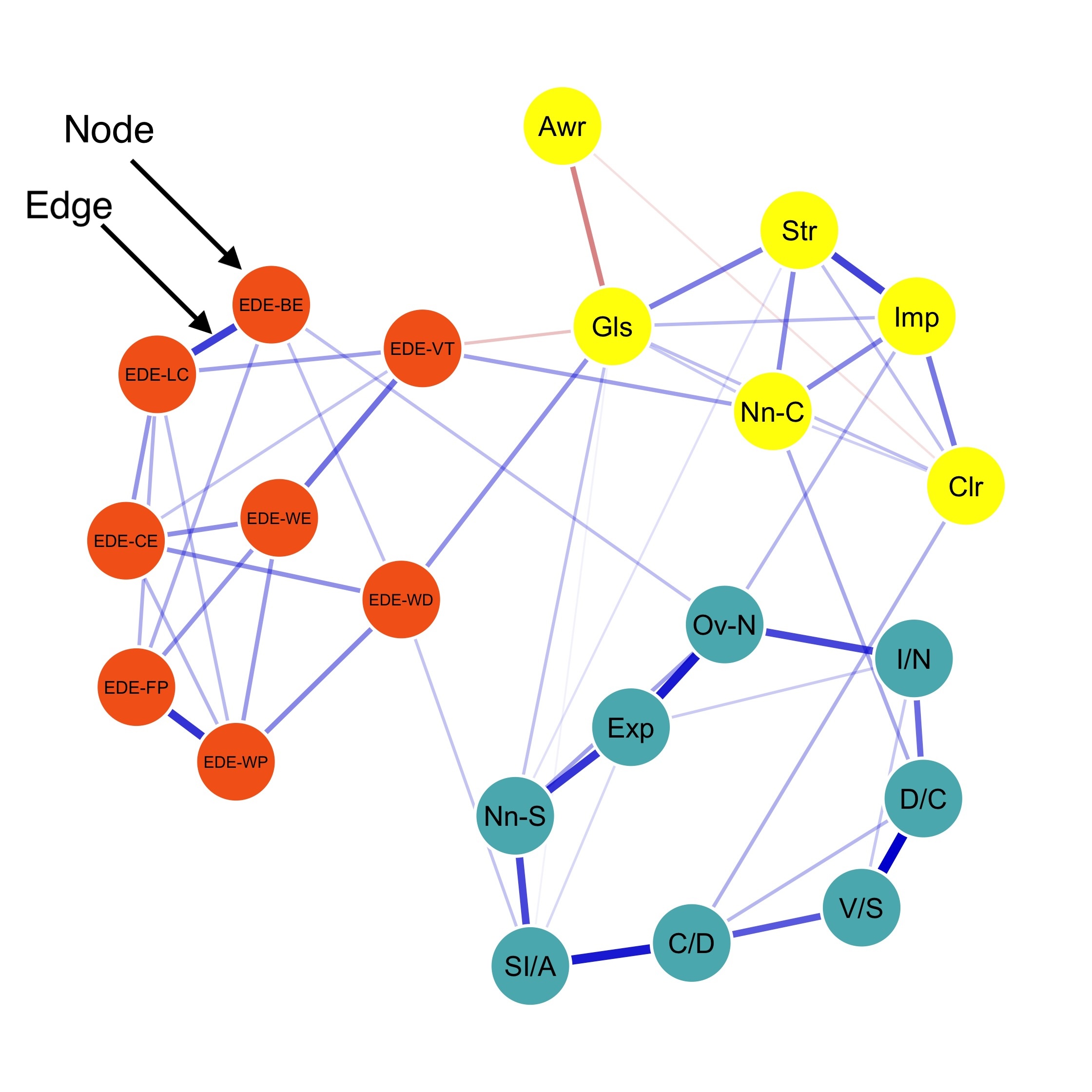
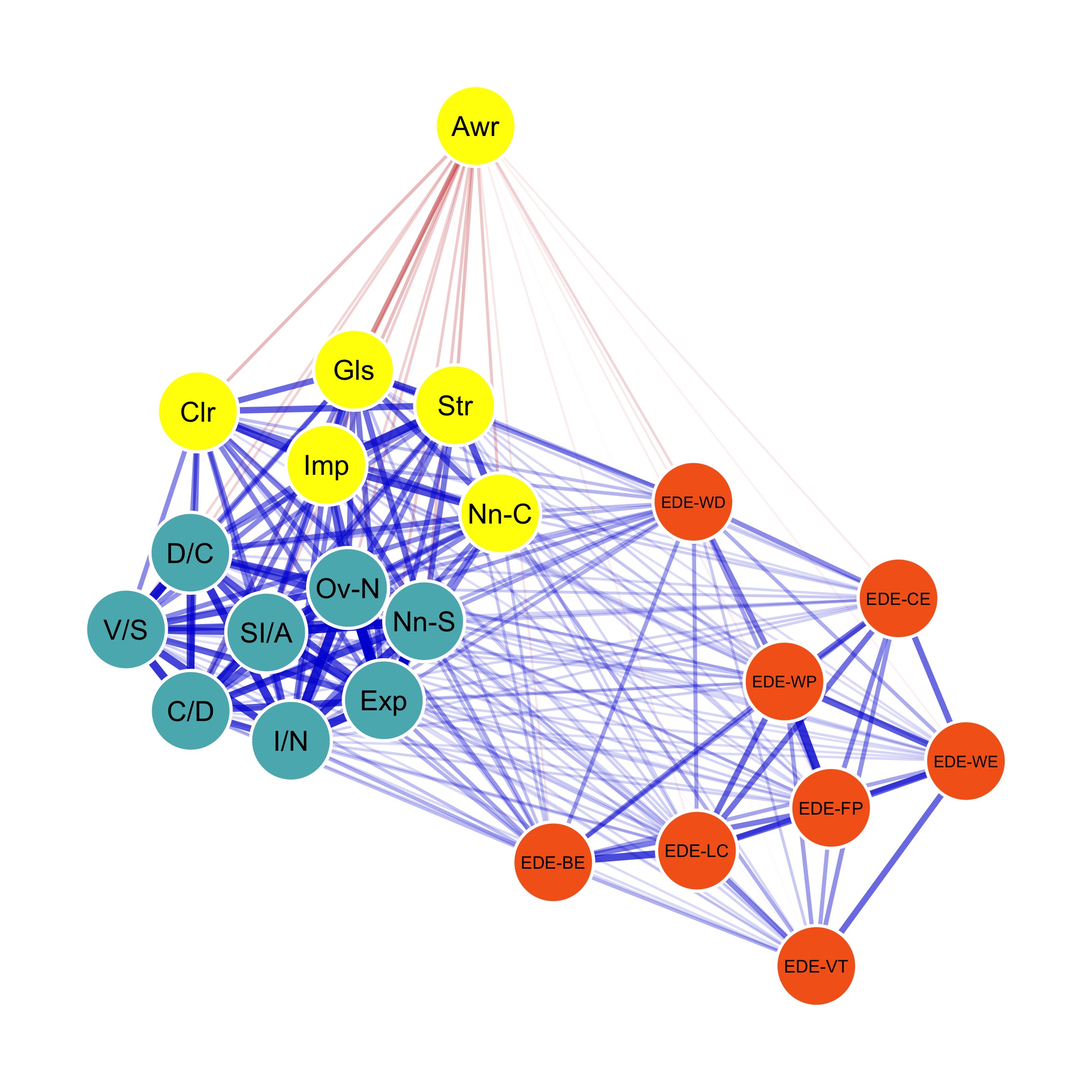
Pyschometric network is exploratory by nature. To obtain a meaningful network structure, psychometric networks need to drop weak edges but keep strong edges.

This procedure is typically called edge selection. One popular edge selection method is regularization.

• Original network structure without regularization is called saturated network; vice versa regularized network

Emotion regulation (Awareness), Interpersonal problems and eating disorder

Workflow of psychometric network

Psychometric network analysis methodology includes steps of network structure estimation (to construct the network), network description (to characterize the network) and network stability analysis (to assess the robustness of results).

Types of data and network models

1. Cross-sectional data (N = large, T = 1)
   • Ising model for categorical variables
   • Gaussian graphical model (GGM; Foygel & Drton, 2010) for continuous variables
   • Mixed graphical model (MGM) for mixed types of variables
2. Panel data (N >> T)
   • Multilevel graphical vector autoregression
     • i.e., longitudinal data, repeated measures
3. Time-series data (\(N \geq 1\), T = large)
   • Graphical vector autoregression
     • i.e., ecological momentary assessment, conducted via smartphones

Network Estimation

Gaussian graphical model

GGM is one type of Pairwise Markov random field (PMRF) when data are continuous.

In a PMRF, the joint likelihood of multivariate data is modelled through the use of pairwise conditional associations, leading to a network representation that is undirected.

For \(p\)-dimensional data following multivariate normal distribution:

\[ \newcommand{\bb}[1]{\boldsymbol{#1}} \bb{X} \sim \mathcal{N}(\mu, \bb{K}^{-1}) \]

Where \(K\) is a inverse covariance matrix of \(\bb{X}\) (\(K = \Sigma^{-1}\)), also known as precision/concentration matrix.

To obtain sparse network structure, the \(i\)th row and \(j\)th column element of \(\bb{K}\), \(k_{ij}=0\) when edge \(\{j, k\}\) is not included in the network \(G\),

• It means \(X^{(i)}\) and \(X^{(j)}\) are independent conditional on the other variables .

Partial correlation networks

GGM can be standardized as the partial correlation network, in which each edge of GGM representing partial correlations between two nodes.

\[ \rho_{ij}=\rho(X^{(i)}, X^{(j)}|\bb{X}^{-(i,j)}) = -\frac{k_{ij}}{\sqrt{k_{ii}}\sqrt{k_{jj}}} \]

Assume there are three variables: fatigue, insomnia, concentration

Sigma = matrix(c(
  1,    -.26,  .31,
  -.26,    1, -.08,
  .31,  -.08,    1  
), ncol = 3, byrow = T)
Sigma

      [,1]  [,2]  [,3]
[1,]  1.00 -0.26  0.31
[2,] -0.26  1.00 -0.08
[3,]  0.31 -0.08  1.00

K = solve(Sigma)
round(K, 2)

      [,1] [,2]  [,3]
[1,]  1.18 0.28 -0.34
[2,]  0.28 1.07  0.00
[3,] -0.34 0.00  1.11

R = K
for (i in 1:nrow(R)) {
  for (j in 1:ncol(R)){
    if (i != j) {
      R[i, j] = - K[i, j] / (sqrt(K[i, i])*sqrt(K[j, j]))
    }else{
      R[i, j] = 1
    }
  }
}
round(R, 2)

      [,1]  [,2] [,3]
[1,]  1.00 -0.25  0.3
[2,] -0.25  1.00  0.0
[3,]  0.30  0.00  1.0

Network Interpretation

1. Someone who is tired is also more likely to suffer from concentration problems and insomnia.
2. Concentration problems and insomnia are conditional independent given the level of fatigue
   • Or the correlation between insomnia and concentration can be totally explained by the relationships of both variables with fatigue

qgraph::qgraph(R, labels = c("Fatigue", "Concentration", "Insomnia"))

Estimation of partial correlation model for cross-sectional data

Factor analysis model:

\[ \bb{X}\sim\mathcal{N}(\mu, \bb{\Lambda\Psi\Lambda^\text{T}+\Phi}) \]

GGM with partial correlation matrix:

\[ \bb{X} \sim \mathcal{N}(0, \bb{\Delta(I-\Omega)^{-1}\Delta}) \]

Where

1. \(\bb{\Delta}\) is a diagonal scaling matrix that controls the variances
2. \(\bb{\Omega}\) is a square symmetrical matrix with \(0\)s on the diagonal and partial correlation coefficients on the off diagonal.

psychonetrics: Partial correlation matrix estimation

Sigma |> round(3)

      [,1]  [,2]  [,3]
[1,]  1.00 -0.26  0.31
[2,] -0.26  1.00 -0.08
[3,]  0.31 -0.08  1.00

R |> round(3)

       [,1]   [,2]  [,3]
[1,]  1.000 -0.248 0.300
[2,] -0.248  1.000 0.001
[3,]  0.300  0.001 1.000

library(psychonetrics)
fit = ggm(covs = Sigma, nobs = 50)
Omega <- fit |> getmatrix("omega") 
Omega |> round(3)# estimated Omega

       [,1]   [,2]  [,3]
[1,]  0.000 -0.248 0.300
[2,] -0.248  0.000 0.001
[3,]  0.300  0.001 0.000

Delta <- fit |> getmatrix('delta') 
Delta |> round(3)

      [,1]  [,2]  [,3]
[1,] 0.921 0.000 0.000
[2,] 0.000 0.966 0.000
[3,] 0.000 0.000 0.951

S = Delta %*% solve(diag(1, 3) - Omega) %*% Delta
S |> round(3)

      [,1]  [,2]  [,3]
[1,]  1.00 -0.26  0.31
[2,] -0.26  1.00 -0.08
[3,]  0.31 -0.08  1.00

BGGM: Bayesian approach

library(BGGM)
set.seed(1234)
dat <- mvtnorm::rmvnorm(500, mean = rep(0, 3), sigma = Sigma)
fit_bggm <- BGGM::estimate(dat, type = "continuous", iter = 1000, analytic = FALSE)
fit_bggm$pcor_mat |> round(3)

       [,1]   [,2]  [,3]
[1,]  0.000 -0.258 0.189
[2,] -0.258  0.000 0.040
[3,]  0.189  0.040 0.000

summary(fit_bggm)

BGGM: Bayesian Gaussian Graphical Models 
--- 
Type: continuous 
Analytic: FALSE 
Formula:  
Posterior Samples: 1000 
Observations (n):
Nodes (p): 3 
Relations: 3 
--- 
Call: 
BGGM::estimate(Y = dat, type = "continuous", analytic = FALSE, 
    iter = 1000)
--- 
Estimates:
 Relation Post.mean Post.sd Cred.lb Cred.ub
     1--2    -0.258   0.042  -0.342  -0.173
     1--3     0.189   0.043   0.105   0.274
     2--3     0.040   0.046  -0.055   0.129
--- 

Edge Selection: Regularization

Multiple procedure and software can be used to perform edge selection:

1. prune function in psychonetrics package uses stepdown model search by pruning non-significant parameters

   • a edge with significance level lower than \(\alpha\) will be removed and re-fit the model until no nonsignificant edge existed
   • \(p\) values of edges needed to be adjusted

2. EBICglasso in qgraph and glasso package uses Extended Bayesian Information Criterion (EBIC) to select best model

   \[ \text{EBIC}=-2\text{L}+E(\log(N))+4\gamma E(log(P)) \]

3. select function in BGGM package uses Bayesian Hypothesis Testing — Bayes Factor (BF) to select model

   • \(\mathcal{H}_0: \rho_{ij}=0\)
   • \(\mathcal{H}_1: \rho_{ij}\in(-1, 1)\)
   • \[ BF = \frac{p(\bb{X}|\mathcal{H}_0)}{p(\bb{X}|\mathcal{H}_1)} \]
   • By default, edges with BF < 3 will be included

Example: Big Five Personality Scale

25 self-reported personality items representing 5 factors.

70.6% edges are nonzero using EBICglasso, while only 63.6% edges are nonzero using BF method and 62.0% edges are kept using \(\alpha =.01\) significance testing

library(psych)
library(qgraph)
data(bfi)
big5groups <- list(
  Agreeableness = 1:5,
  Conscientiousness = 6:10,
  Extraversion = 11:15,
  Neuroticism = 16:20,
  Openness = 21:25
)
CorMat <- cor_auto(bfi[,1:25])

EBICgraph <- EBICglasso(CorMat, nrow(bfi), 0.5, threshold = TRUE)

## density
density_nonzero_edge <- function(pcor_matrix){
  N_nonzero_edge = (sum(pcor_matrix == 0) - ncol(pcor_matrix)) /2
  N_all_edge = ncol(pcor_matrix)*(ncol(pcor_matrix)-1)/2
  N_nonzero_edge/N_all_edge
}
density_nonzero_edge(EBICgraph)

[1] 0.7066667

PruneFit <- ggm(bfi[,1:25]) |> prune(alpha = .01)
density_nonzero_edge(getmatrix(PruneFit, "omega"))

[1] 0.62

BGGMfit <- BGGM::explore(bfi[,1:25], type = "continuous", iter = 1000, analytic = FALSE) |> 
  select()
density_nonzero_edge(BGGMfit$pcor_mat_zero)

[1] 0.62

Network Structure

EBICglasso

Sig. Test

BF

Centrality - Strength

Strength centrality measures suggest that C4 and E4 or N1 have highest centrality indicating they play most imporatant roles in the networks.

Method 1: EBICglasso

Method 2: Sig. Test

Method 3: Bayes Factor

Centrality - Bridge

E4 and E5 has highest bridge strength, indicating they serve as bridges linking communities of personality. They are important elements connecting varied types of personality

Method 1: EBICglasso

Method 2: Sig. Test

Method 3: Bayes Factor

Wrapping up

1. Network analysis is an alternative way of modeling dependency among variables.
2. Gaussian graphical model is used for multivariate continuous data.
3. The goal is to estimate network structure, node importance, and stability.

Other Materials:

1. Jihong’s post: how to choose network analysis estimation

Reference

Kan, Kees-Jan, Han L. J. van der Maas, and Stephen Z. Levine. 2019. “Extending Psychometric Network Analysis: Empirical Evidence Against g in Favor of Mutualism?” Intelligence 73 (March): 52–62. https://doi.org/10.1016/j.intell.2018.12.004.