Lecture 04: Distribution and Estimation

Jihong Zhang*, Ph.D

Educational Statistics and Research Methods (ESRM) Program*

University of Arkansas

2024-09-16

Today’s Class

• Review Homework 1

• The building blocks: The basics of mathematical statistics:

  • Random variables: Definition & Types

  • Univariate distribution

    • General terminology (e.g., sufficient statistics)

    • Univariate normal (aka Gaussian)

    • Other widely used univariate distributions

  • Types of distributions: Marginal | Conditional | Joint

  • Expected values: means, variances, and the algebra of expectations

  • Linear combinations of random variables

• The finished product: How the GLM fits within statistics

  • The GLM with the normal distribution

  • The statistical assumptions of the GLM

  • How to assess these assumptions

ESRM 64503: Homework 1

Question 2

• Copy and paste your R syntax and R output that calculates the group Senior-Old’s standard error of group mean (use the data and model we’ve used in class).

  • Aim: Test whether the group mean of senior-old significantly higher than the baseline (here, 0 score)

\[ \mathbf{Test = \beta_0 +\beta_1Senior + \beta_2New +\beta_3Senior*New} \]

• The group mean of Senior-Old is \(\beta_0 + \beta_1\).

• Based on algebra for variance, we know hat

\[ Var(\beta_0 + \beta_1) = Var(\beta_0)+Var(\beta_1) +2*Cov(\beta_0, \beta_1) \]

• vcor function provides the variances and covaraicnes for \(\beta_0\), \(\beta_1\), \(\beta_2\), and \(\beta_3\)

# R syntax
library(ESRM64503)
library(tidyverse)
model1 <- lm(Test ~ Senior + New + Senior * New, data = dataTestExperiment)
data("dataTestExperiment")
Var_beta_0 <- vcov(model1)[1,1]
Var_beta_1 <- vcov(model1)[2,2]
Cov_beta_0_1 <- vcov(model1)[1,2]
Var_Test_SeniorOld <- Var_beta_0 + Var_beta_1 + 2*Cov_beta_0_1
(SE_Test_SeniorOld <- sqrt(Var_Test_SeniorOld)) 

[1] 0.5364078

Question 3

• Copy and paste your R syntax and R output that calculates the standard error of conditional main effect of New (New vs. Old) when Senior = 1.

  • Aim: Test whether the conditional main effect of New when Senior significantly different from 0
    • In other words, when individuals are senior, whether new or old instruction method has significantly differences in their test scores

\[ \beta_{2|Senior =1} = \beta_2 + \beta_3 * 1 \]

• Based on algebra for variance, we know that

\[ Var(\beta_2 + \beta_3) = Var(\beta_2)+Var(\beta_3) +2*Cov(\beta_2, \beta_3) \]

• vcor function provides the variances and covariances for \(\beta_0\), \(\beta_1\), \(\beta_2\), and \(\beta_3\)

# R syntax
Var_beta_2 <- vcov(model1)[3,3]
Var_beta_3 <- vcov(model1)[4,4]
Cov_beta_2_3 <- vcov(model1)[3,4]
Var_betaofNew_Senior1 <- Var_beta_2 + Var_beta_3 + 2*Cov_beta_2_3
(SE_betaofNew_Senior1 <- sqrt(Var_betaofNew_Senior1)) 

[1] 0.7585952

Unit 1: Random Variables & Statistical Distribution

Definition of Random Variables

• Random: situations in which the certainty of the outcome is unknown and is at least in part due to chance

• Variable: a value that may change give the scope of a given problem or set of operations

• Random Variable: a variable whose outcome depends on chance (possible values might represent the possible outcomes of a yet-to-be performed experiment)

Today, we will denote a random variable with a lower-cased: x

Question: which one in the following options is random variable:

1. any company’s revenue in 2024

2. one specific company’s monthly revenue in 2024

3. companies whose revenue over than $30 billions

My answer: only (a)

Types of Random Variables

1. Continuous
   • Examples of continuous random variables:
     • x represent the height of a person, draw at random
     • Y (the outcome/DV in a GLM)
     • Some variables like exam score or motivation scores are not “true” continuous variables, but it is convenient to consider them as “continuous”
2. Discrete (also called categorical, generally)
   • Example of discrete random variables:
     • x represents the gender of a person, drawn at random
     • Y (outcomes like yes/no; pass/not pass; master / not master a skill; survive / die)
3. Mixture of Continuous and Discrete:
   • Example of mixture: \[\begin{equation} x = \begin{cases} RT & \text{between 0 and 45 seconds} \\ 0 & \text{otherwise} \end{cases} \end{equation}\]

Key Features of Random Variable

1. Random variables each are described by a probability density / mass function (PDF) – \(f(x)\)

   • PDF indicates relative frequency of occurrence

   • A PDF is a math function that gives rough picture of the distribution from which a random variable is draw

2. The type of random variable dictates the name and nature of these functions:

   • Continuous random variables:

     • \(f(x)\) is called a probability density function

     • Area under curve must equal to 1 (found by calculus integration)

     • Height of curve (the function value \(f(x)\)):

       • Can be any positive number

       • Reflects relative likelihood of an observation occurring

   • Discrete random variables:

     • \(f(x)\) is called a probability mass function

     • Sum across all values must equal 1

Note

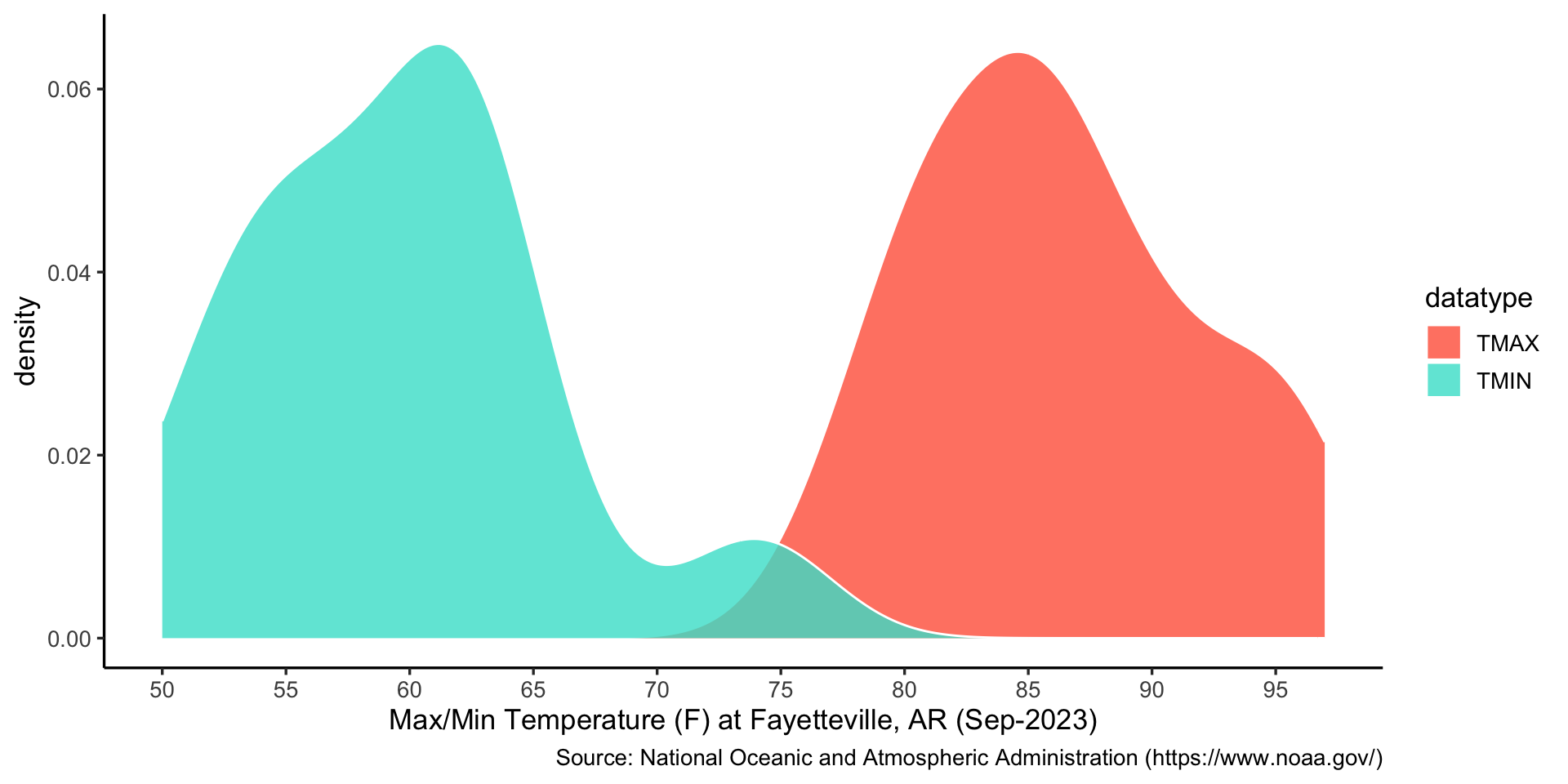
Both max and min values of temperature can be considered as continuous random variables.

• Question 1: what are the probabilities of integrating all values of max and min temperatures ({1, 1} or {0.5, 0.5})

• Answer: it is {1, 1} for max and min temperatures. Because they are two separated random variables.

library(tidyverse)
temp <- read.csv("data/temp_fayetteville.csv")
temp$value_F <- (temp$value / 10 * 1.8) + 32
temp |> 
  ggplot() +
  geom_density(aes(x = value_F, fill = datatype), col = "white", alpha = .8) +
  labs(x = "Max/Min Temperature (F) at Fayetteville, AR (Sep-2023)", 
       caption = "Source: National Oceanic and Atmospheric Administration (https://www.noaa.gov/)") +
  scale_x_continuous(breaks = seq(min(temp$value_F), max(temp$value_F), by = 5)) +
  scale_fill_manual(values = c("tomato", "turquoise")) +
  theme_classic(base_size = 13) 

Other key Terms

• The sample space is the set of all values that a random variable x can take:
  • Example 1: The sample space for a random variable x from a normal distribution \(x \sim N(\mu_x, \sigma^2_x)\) is \((-\infty, +\infty)\).
  • Example 2: The sample space for a random variable x representing the outcome of a coin flip is {H, T}
  • Example 3: The sample space for a random variable x representing the outcome of a roll of a die is {1, 2, 3, 4, 5, 6}
• When using generalized models, the trick is to pick a distribution with a sample space that matches the range of values obtainable by data
  • Logistic regression - Match Bernoulli distribution (Example 2)
  • Poisson regression - Match Poisson distribution (Example 3)

Uses of Distributions in Data Analysis

• Statistical models make distributional assumptions on various parameters and / or parts of data

• These assumptions govern:

  • How models are estimated

  • How inferences are made

  • How missing data may be imputed

• If data do not follow an assumed distribution, inferences may be inaccurate

  • Sometimes a very big problem, other times not so much

• Therefore, it can be helpful to check distributional assumptions prior to running statistical analysis

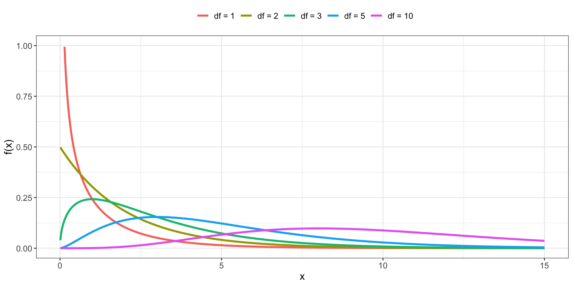
Continuous Univariate distributions

• To demonstrate how continuous distributions work and look, we will discuss three:

  • Uniform distribution

  • Normal distribution

  • Chi-square distribution

• Each are described a set of parameters, which we will later see are what give us our inferences when we analysis data

• What we then do is put constraints on those parameters based on hypothesized effects in data

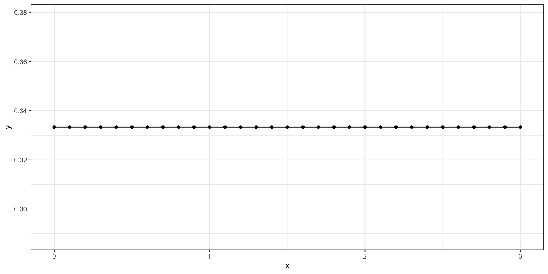
Uniform distribution

• The uniform distribution is how to help set up how continuous distributions work

  • Typically, used for simulation studies that parameters are randomly generated

• For a continuous random variable x that ranges from (a, b), the uniform probability density function is:

  \(f(x) = \frac{1}{b-a}\)

• The uniform distribution has two parameters

  x = seq(0, 3, .1)
  y = dunif(x, min = 0, max = 3)
  ggplot() +
    geom_point(aes(x = x, y = y)) +
    geom_path(aes(x = x, y = y)) +
    theme_bw()

#| standalone: true
#| viewerHeight: 800
library(shiny)
library(bslib)
library(ggplot2)
library(dplyr)
library(tidyr)
set.seed(1234)
# Define UI for application that draws a histogram
ui <- fluidPage(
  
  # Application title
  titlePanel("Uniform distribution"),
  
  # Sidebar with a slider input for number of bins 
  sidebarLayout(
    sidebarPanel(
      sliderInput("a",
                  "Lower Bound (a):",
                  min = 1,
                  max = 20,
                  value = 1,
                  animate = animationOptions(interval = 5000, loop = TRUE)),
      uiOutput("b_slider")
    ),
    
    # Show a plot of the generated distribution
    mainPanel(
      plotOutput("distPlot")
    )
  )
)

# Define server logic required to draw a histogram
x <- seq(0, 40, .02)
server <- function(input, output) {
  observeEvent(input$a, {
    output$b_slider <<- renderUI({
      sliderInput("b",
                  "Upper Bound (b):",
                  min = as.numeric(input$a),
                  max = 40,
                  value = as.numeric(input$a) + 1)
    })
    # browser()
    y <<- reactive({dunif(x, min = as.numeric(input$a), max = as.numeric(input$b))})
  })
  # browser()
  observe({
    output$distPlot <- renderPlot({
      # generate bins based on input$bins from ui.R
      ggplot() +
        aes(x = x, y = y())+
        geom_point() +
        geom_path() +
        labs(x = "x", y = "probability") +
        theme_bw() +
        theme(text = element_text(size = 20))
    })
  })
}

# Run the application 
shinyApp(ui = ui, server = server)

More on the Uniform Distribution

• To demonstrate how PDFs work, we will try a few values:

conditions <- tribble(
   ~x, ~a, ~b,
   .5,  0,  1,
  .75,  0,  1,
   15,  0, 20,
   15, 10, 20
) |> 
  mutate(y = dunif(x, min = a, max = b))
conditions

# A tibble: 4 × 4
      x     a     b     y
  <dbl> <dbl> <dbl> <dbl>
1  0.5      0     1  1   
2  0.75     0     1  1   
3 15        0    20  0.05
4 15       10    20  0.1 

• The uniform PDF has the feature that all values of x are equally likely across the sample space of the distribution
  • Therefore, you do not see x in the PDF \(f(x)\)
• The mean of the uniform distribution is \(\frac{1}{2}(a+b)\)
• The variance of the uniform distribution is \(\frac{1}{12}(b-a)^2\)

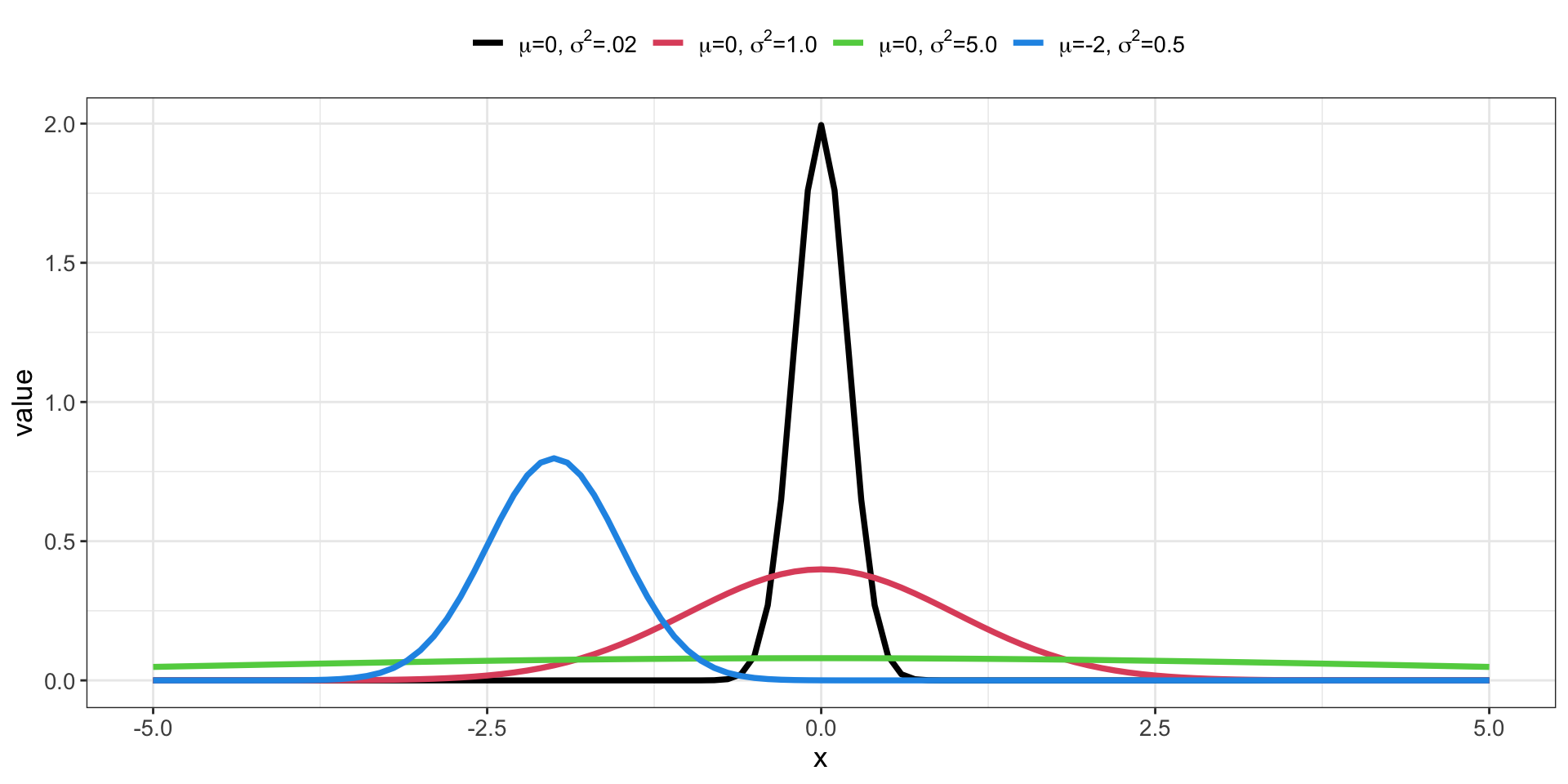
Univariate Normal Distribution

• For a continuous random variable x (ranging from \(-\infty\) to \(\infty\)), the univariate normal distribution function is:

\[ f(x) = \frac1{\sqrt{2\pi\sigma^2_x}}\exp(-\frac{(x-\mu_x)^2}{2\sigma^2_x}) \]

• The shape of the distribution is governed by two parameters:

  • The mean \(\mu_x\)

  • The variance \(\sigma^2_x\)

  • These parameters are called sufficient statistics (they contain all the information about the distribution)

• The skewness (lean) and kurtosis (peakedness) are fixed

• Standard notation for normal distributions is \(x\sim N(\mu_x, \sigma^2_x)\)

  • Read as: “x follows a normal distribution with a mean \(\mu_x\) and a variance \(\sigma^2_x\)”

• Linear combinations of random variables following normal distributions result in a random variable that is normally distributed

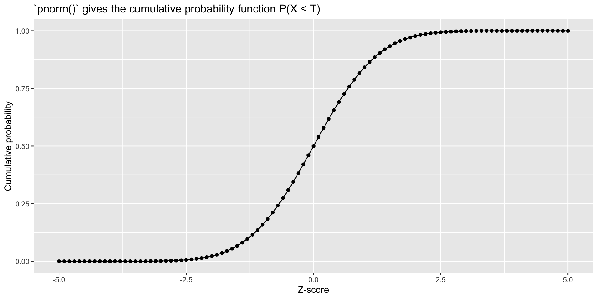
Univariate Normal Distribution in R: pnorm

Density (dnorm), distribution function (pnorm), quantile function (qnorm) and random generation (rnorm) for the normal distribution with mean equal to mean and standard deviation equal to sd.

Z = seq(-5, 5, .1) # Z-score
ggplot() +
  aes(x = Z, y = pnorm(q = Z, lower.tail = TRUE)) +
  geom_point() +
  geom_path() +
  labs(x = "Z-score", y = "Cumulative probability",
       title = "`pnorm()` gives the cumulative probability function P(X < T)")

Univariate Normal Distribution in R: dnorm

x <- seq(-5, 5, .1)

params <- list(
  y_set1 = c(mu =  0, sigma2 = 0.2),
  y_set2 = c(mu =  0, sigma2 = 1.0),
  y_set3 = c(mu =  0, sigma2 = 5.0),
  y_set4 = c(mu = -2, sigma2 = 0.5)
)

y <- sapply(params, function(param) dnorm(x, mean = param['mu'], sd = param['sigma2']))

dt <- cbind(x, y) |> 
  as.data.frame() |> 
  pivot_longer(starts_with("y_"))

ggplot(dt) +
  geom_path(aes(x = x, y = value, color = name, group = name), linewidth = 1.3) +
  scale_color_manual(values = 1:4,
                     name = "",
                     labels = c('y_set1' = expression(mu*"=0, "*sigma^2*"=.02"),
                                'y_set2' = expression(mu*"=0, "*sigma^2*"=1.0"),
                                'y_set3' = expression(mu*"=0, "*sigma^2*"=5.0"),
                                'y_set4' = expression(mu*"=-2, "*sigma^2*"=0.5"))
                     ) +
  theme_bw() +
  theme(legend.position = "top", text = element_text(size = 13))

Chi-Square Distribution

• Another frequently used univariate distribution is the Chi-square distribution

  • Sampling distribution of the variance follows a chi-square distribution

  • Likelihood ratios follow a chi-square distribution

• For a continuous random variable x (ranging from 0 to \(\infty\)), the chi-square distribution is given by:

  \[ f(x) =\frac1{2^{\frac{\upsilon}{2}} \Gamma(\frac{\upsilon}{2})} x^{\frac{\upsilon}{2}-1} \exp(-\frac{x}2) \]

• \(\Gamma(\cdot)\) is called the gamma function

• The chi-square distribution is govern by one parameter: \(\upsilon\) (the degrees of freedom)

  • The mean is equal to \(\upsilon\); the variance is equal to 2\(\upsilon\)

x <- seq(0.01, 15, .01)
df <- c(1, 2, 3, 5, 10)
dt2 <- as.data.frame(sapply(df, \(df) dchisq(x, df = df)))
dt2_with_x <- cbind(x = x, dt2)
dt2_with_x |> 
  pivot_longer(starts_with("V")) |> 
  ggplot() +
  geom_path(aes(x = x, y = value, color = name), linewidth = 1.2) +
  scale_y_continuous(limits = c(0, 1)) +
  scale_color_discrete(name = "", labels = paste("df =", df)) +
  labs(y = "f(x)") +
  theme_bw() +
  theme(legend.position = "top", text = element_text(size = 13))

#| standalone: true
#| viewerHeight: 800
library(shiny)
library(bslib)
library(ggplot2)
library(dplyr)
library(tidyr)
set.seed(1234)
# Define UI for application that draws a histogram
ui <- fluidPage(

    # Application title
    titlePanel("Chi-square distribution"),

    # Sidebar with a slider input for number of bins 
    sidebarLayout(
        sidebarPanel(
            sliderInput("Df",
                        "Degree of freedom:",
                        min = 1,
                        max = 20,
                        value = 1,
                        animate = animationOptions(interval = 5000, loop = TRUE)),
           verbatimTextOutput(outputId = "Df_display")
        ),

        # Show a plot of the generated distribution
        mainPanel(
           plotOutput("distPlot")
        )
    )
)

# Define server logic required to draw a histogram
server <- function(input, output) {
    x <- seq(0.01, 15, .01)
    df <- reactive({input$Df}) 
    
    output$Df_display <- renderText({
        paste0("DF = ", df())
    })
    output$distPlot <- renderPlot({
        # generate bins based on input$bins from ui.R
        
        
        dt2 <- as.data.frame(sapply(df(), \(df) dchisq(x, df = df)))
        dt2_with_x <- cbind(x = x, dt2)
        dt2_with_x |> 
            pivot_longer(starts_with("V")) |> 
            ggplot() +
            geom_path(aes(x = x, y = value), linewidth = 1.2) +
            scale_y_continuous(limits = c(0, 1)) +
            labs(y = "f(x)") +
            theme_bw() +
            theme(legend.position = "top", text = element_text(size = 13))
    })
}

# Run the application 
shinyApp(ui = ui, server = server)

Marginal, Joint, And Conditional Distribution

Moving from One to Multiple Random Variables

• When more than one random variable is present, there are several different types of statistical distributions:

• We will first consider two discrete random variables：

  • x is the outcome of the flip of a penny {\(H_p\), \(T_p\)}

    • \(f(x=H_p) = .5\); \(f(x =T_p) = .5\)

  • z is the outcome of the flip of a dime {\(H_d\), \(T_d\)}

    • \(f(z=H_p) = .5\); \(f(z =T_p) = .5\)

• We will consider the following distributions:

  • Marginal distribution

    • The distribution of one variable only (either \(f(x)\) or \(f(z)\))

  • Joint distribution

    • \(f(x, z)\): the distribution of both variables (both x and z)

  • Conditional distribution

    • The distribution of one variable, conditional on values of the other:

      • \(f(x|z)\): the distribution of x given z

      • \(f(z|x)\): the distribution of z given x

Marginal Distribution

• Marginal distributions are what we have worked with exclusively up to this point: they represent the distribution by itself

  • Continuous univariate distributions

  • Categorical distributions

    • The flip of a penny

    • The flip of a dime

Joint Distribution

• Joint distributions describe the distribution of more than one variable, simultaneously

  • Representations of multiple variables collected

• Commonly, the joint distribution function is denoted with all random variables separated by commas

  • In our example, \(f(x,z)\) is the joint distribution of the outcome of flipping both a penny and a dime

    • As both are discrete, the joint distribution has four possible values:

      (1) \(f(x = H_p,z=H_d)\) (2) \(f(x = H_p,z=T_d)\) (3) \(f(x = T_p,z=H_d)\) (4) \(f(x = T_p,z=T_d)\)

• Joint distributions are multivariate distributions

• We will use joint distributions to introduce two topics

  • Joint distributions of independent variables

  • Joint distributions – used in maximum likelihood estimation

Joint Distributions of Independent Random Variables

• Random variables are said to be independent if the occurrence of one event makes it neither more nor less probable of another event

  • For joint distributions, this means: \(f(x,z)=f(x)f(z)\)

• In our example, flipping a penny and flipping a dime are independent – so we can complete the following table of their joint distribution:

  	z = \(H_d\)	z = \(T_d\)	Marginal (Penny)
  \(x = H_p\)	\(\color{tomato}{f(x=H_p, z=H_d)}\)	\(\color{tomato}{f(x=H_p, z=T_d)}\)	\(\color{turquoise}{f(z=H_p)}\)
  \(x = T_p\)	\(\color{tomato}{f(x= T_p, z=H_d)}\)	\(\color{tomato}{f(x=T_p, z=T_d)}\)	\(\color{turquoise}{f(z=T_d)}\)
  Marginal (Dime)	\(\color{turquoise}{f(z=H_d)}\)	\(\color{turquoise}{f(z=T_d)}\)

Joint Distributions of Independent Random Variables

• Because the coin flips are independent, this because:

	z = \(H_d\)	z = \(T_d\)	Marginal (Penny)
\(x = H_p\)	\(\color{tomato}{f(x=H_p)f( z=H_d)}\)	\(\color{tomato}{f(x=H_p)f( z=T_d)}\)	\(\color{turquoise}{f(z=H_p)}\)
\(x = T_p\)	\(\color{tomato}{f(x= T_p)f( z=H_d)}\)	\(\color{tomato}{f(x=T_p)f( z=T_d)}\)	\(\color{turquoise}{f(z=T_d)}\)
Marginal (Dime)	\(\color{turquoise}{f(z=H_d)}\)	\(\color{turquoise}{f(z=T_d)}\)

• Then, with numbers:

	z = \(H_d\)	z = \(T_d\)	Marginal (Penny)
\(x = H_p\)	\(\color{tomato}{.25}\)	\(\color{tomato}{.25}\)	\(\color{turquoise}{.5}\)
\(x = T_p\)	\(\color{tomato}{.25}\)	\(\color{tomato}{.25}\)	\(\color{turquoise}{.5}\)
Marginal (Dime)	\(\color{turquoise}{.5}\)	\(\color{turquoise}{.5}\)

Marginalizing Across a Joint Distribution

• If you had a joint distribution, \(\color{orchid}{f(x, z)}\), but wanted the marginal distribution of either variable (\(f(x)\) or \(f(z)\)) you would have to marginalize across one dimension of the joint distribution.

• For categorical random variables, marginalize = sum across every value of z

\[ f(x) = \sum_zf(x, z) \]

• For example, \(f(x = H_p) = f(x = H_p, z=H_d) +f(x = H_p, z=T_d)=.5\)

• For continuous random variables, marginalize = integrate across z

  • The integral:

    \[ f(x) = \int_zf(x,z)dz \]

Conditional Distributions

• For two random variables x and z, a conditional distribution is written as: \(f(z|x)\)

  • The distribution of z given x

• The conditional distribution is equal to the joint distribution divided by the marginal distribution of the conditioning random variable

  \[ f(z|x) = \frac{f(z,x)}{f(x)} \]

• Conditional distributions are found everywhere in statistics

  • The general linear model uses the conditional distribution variable

    \[ Y \sim N(\beta_0+\beta_1X, \sigma^2_e) \]

Example: Conditional Distribution

• For two discrete random variables with {0, 1} values, the conditional distribution can be shown in a contingency table:

	z = \(H_d\)	z = \(T_d\)	Marginal (Penny)
\(x = H_p\)	\(\color{tomato}{.25}\)	\(\color{tomato}{.25}\)	\(\color{turquoise}{.5}\)
\(x = T_p\)	\(\color{tomato}{.25}\)	\(\color{tomato}{.25}\)	\(\color{turquoise}{.5}\)
Marginal (Dime)	\(\color{turquoise}{.5}\)	\(\color{turquoise}{.5}\)

Conditional: \(f(z | x= H_p)\):

\(f(z=H_d|x =H_p) = \frac{f(z=H_d, x=H_p}{f(x = H_p)} = \frac{.25}{.5}=.5\)

\(f(z = T_d | x = H_p)= \frac{f(z=T_d, x=H_p}{f(x=H_p)} = \frac{.25}{.5} = .5\)

Expected Values and The Algebra of Expectation

Expected Values

• Expected values are statistics taken the sample space of a random variable: they are essentially weighted averages

  set.seed(1234)
  x = rnorm(100, mean = 0, sd = 1)
  weights = dnorm(x, mean = 0, sd = 1)
  mean(weights * x)

  [1] -0.05567835

• The weights used in computing this average correspond to the probabilities (for a discrete random variable) or to the densities (for a continuous random variable)

Note

The expected value is represented by \(E(x)\)

The actual statistic that is being weighted by the PDF is put into the parenthesis where x is now

• Expected values allow us to understand what a statistical model implies about data, for instance:

  • How a GLM specifies the (conditional) mean and variance of a DV

Expected Value Calculation

• For discrete random variables, the expected value is found by:

  \[ E(x) = \sum_x xP(X=x) \]

• For example, the expected value of a roll of a die is:

  \[ E(x) = (1)\frac16+ (2)\frac16+(3)\frac16+(4)\frac16+(5)\frac16+6\frac16 \]

• For continuous random variables, the expected value is found by

  \[ E(x) = \int_x xf(x)dx \]

• We won’t be calculating theoretical expected values with calculus… we use them only to see how models imply things about out data

Variance and Covariance… As Expected Values

• A distribution’s theoretical variance can also be written as an expected value:

  \[ V(x) = E(x-E(x))^2 = E(x -\mu_x)^2 \]

  • This formula helps us understand predictions made by GLMs and how that corresponds to statistical parameters we interpret

• For a roll of a die, the theoretical variance is:

  \[ V(x) = E(x - 3.5)^2 = \frac16(1-3.5)^2 + \frac16(2-3.5)^2 + \frac16(3-3.5)^2 + \frac16(4-3.5)^2 + \frac16(5-3.5)^2 + \frac16(6-3.5)^2 = 2.92 \]

• Likewise, for a pair of random variable x and z, the covariance can be found from their joint distributions:

  \[ \text{Cov}(x,z)=E(xz)-E(x)E(z) = E(xz)-\mu_x\mu_z \]

  set.seed(1234)
  N = 100
  x = rnorm(N, 2, 1)
  z = rnorm(N, 3, 1)
  xz = x*z
  (Cov_xz = mean(xz)-mean(x)*mean(z)) / ((N-1)/N) # unbiased covariance
  cov(x, z)

  [1] -0.02631528
  [1] -0.02631528

Linear Combination of Random Variables

Linear Combinations of Random Variables

• A linear combination is an expression constructed from a set of terms by multiplying each term by a constant and then adding the results \[ x = c + a_1z_1+a_2z_2+a_3z_3 +\cdots+a_nz_n \]

• More generally, linear combinations of random variables have specific implications for the mean, variance, and possibly covariance of the new random variable

• As such, there are predicable ways in which the means, variances, and covariances change

Algebra of Expectations

• Sums of Constants

\[ E(x+c) = E(x)+c \\ \text{Var}(x+c) = \text{Var}(x) \\ \text{Cov}(x+c, z) = \text{Cov}(x, z) \]

Example

Imagine for weight variable, each individual increases 3 lbs:

set.seed(1234)
library(ESRM64503)
x = dataSexHeightWeight$weightLB
c_ = 3
z = dataSexHeightWeight$heightIN
mean(x + c_); mean(x)+c_

[1] 186.4

[1] 186.4

var(x + c_); var(x)

[1] 3179.095

[1] 3179.095

cov(x, z); cov(x+c_, z) # decimal place issue, near() accepts two values' diff less than .00001

[1] 334.8316

[1] 334.8316

• Products of Constants:

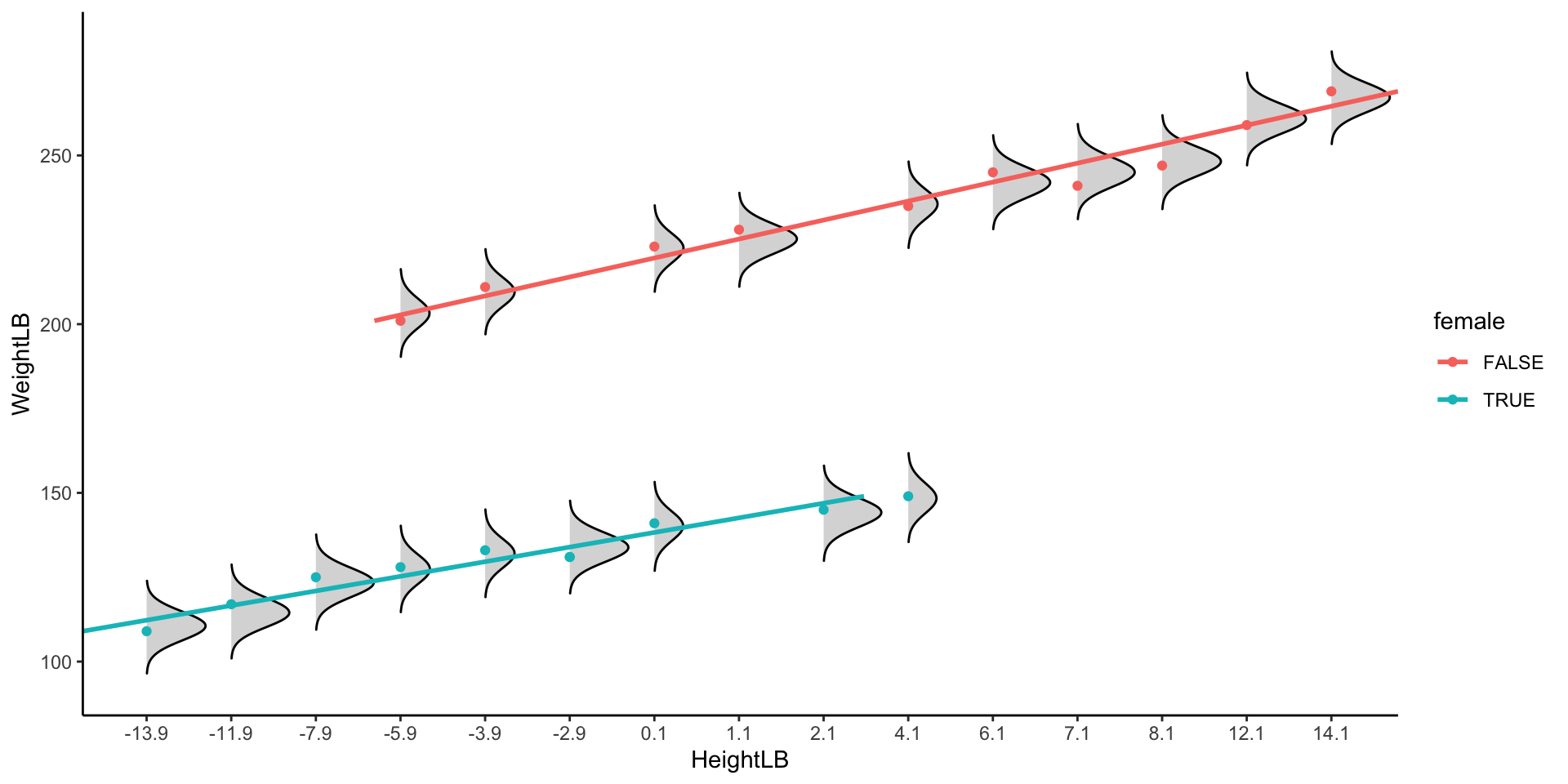
\[ E(cx) = cE(x) \\ \text{Var}(cx) = c^2\text{Var}(x) \\ \text{Cov}(cx, dz) = c*d*\text{Cov}(x, z) \] Imagine you wanted to convert weight from pounds to kilograms (where 1 pound = .453 kg) and convert height from inches to cm (where 1 inch = 2.54 cm)

c_ = .453
mean(x*c_); mean(x)*c_

[1] 83.0802

[1] 83.0802

var(x*c_); var(x)*c_^2

[1] 652.3789

[1] 652.3789

d_ = 2.54
cov(c_*x, d_*z);c_*d_*cov(x, z)

[1] 385.2639

[1] 385.2639

• Sums of Multiple Random Variables:

\[ E(cx+dz) = cE(x) + dE(z) \\ \text{Var}(cx+dz) = c^2\text{Var}(x) + d^2\text{Var}(z) + 2c*d*\text{Cov}(x,z)\\ \]

mean(x*c_+z*d_); mean(x)*c_+mean(z)*d_

[1] 255.5462

[1] 255.5462

var(x*c_+z*d_); c_^2*var(x) + d_^2*var(z) + 2*c_*d_*cov(x, z)

[1] 1780.054

[1] 1780.054

Where We Use This Algebra

• Remember how we calculated the standard error of conditional main effect from simple main effect and interaction effect

\[ \mathbf{Test = 82.20 + 2.16*Senior + 7.76*New - 3.04*Senior*New} \]

• Conditional Main Effects of Senior When New is 1 is (2.16 - 3.04) = -0.88

  • We know that \(Var(\beta_{Senior})\) is 0.575, \(Var(\beta_{Senior*New})\) is 1.151, and \(Cov(\beta_{Senior}, \beta_{Senior*New})\) is -0.575.

model1 <- lm(Test ~ Senior + New + Senior * New, data = dataTestExperiment)
vcov(model1)

            (Intercept)     Senior        New Senior:New
(Intercept)   0.2877333 -0.2877333 -0.2877333  0.2877333
Senior       -0.2877333  0.5754667  0.2877333 -0.5754667
New          -0.2877333  0.2877333  0.5754667 -0.5754667
Senior:New    0.2877333 -0.5754667 -0.5754667  1.1509333

Then,

\[ \mathbf{Var(\beta_{Senior}+\beta_{Senior*New}) = Var(\beta_{Senior}) + Var(\beta_{Senior*New}) + 2Cov(\beta_{Senior},\beta_{Senior*New}) \\ = 0.575 + 1.151 - 2* 0.575 = 0.576} \] Thus, \(SE(\beta_{Senior}+\beta_{Senior*New})=0.759\)

Combining the GLM with Expections

• Using the algebra of expectations predicting Y from X and Z:

\[ \hat{Y}_p=E(Y_p)=E(\beta_0+\beta_1X_p+\beta_2Z_p+\beta_3X_pZ_p+e_p) \\ = \beta_0+\beta_1X_p+\beta_2Z_p+\beta_3X_pZ_p+E(e_p) \\ = \beta_0+\beta_1X_p+\beta_2Z_p+\beta_3X_pZ_p \]

• The variance of \(f(Y_p|X_p, Z_p)\):

\[ V(Y_P)=V(\beta_0+\beta_1X_p+\beta_2Z_p+\beta_3X_pZ_p+e_p)\\ = V(e_p)=\sigma_e^2 \]

Examining What This Means in the Context of Data

• If you recall from the regression analysis of the height/weight data, the final model we decided to interpret: Model 5

\[ W_p = \beta_0+\beta_1 (H_p-\bar{H}) +\beta_2F_p+\beta_3 (H_p-\bar{H}) F_p + e_p \]

where \(e_p \sim N(0, \sigma_e^2)\)

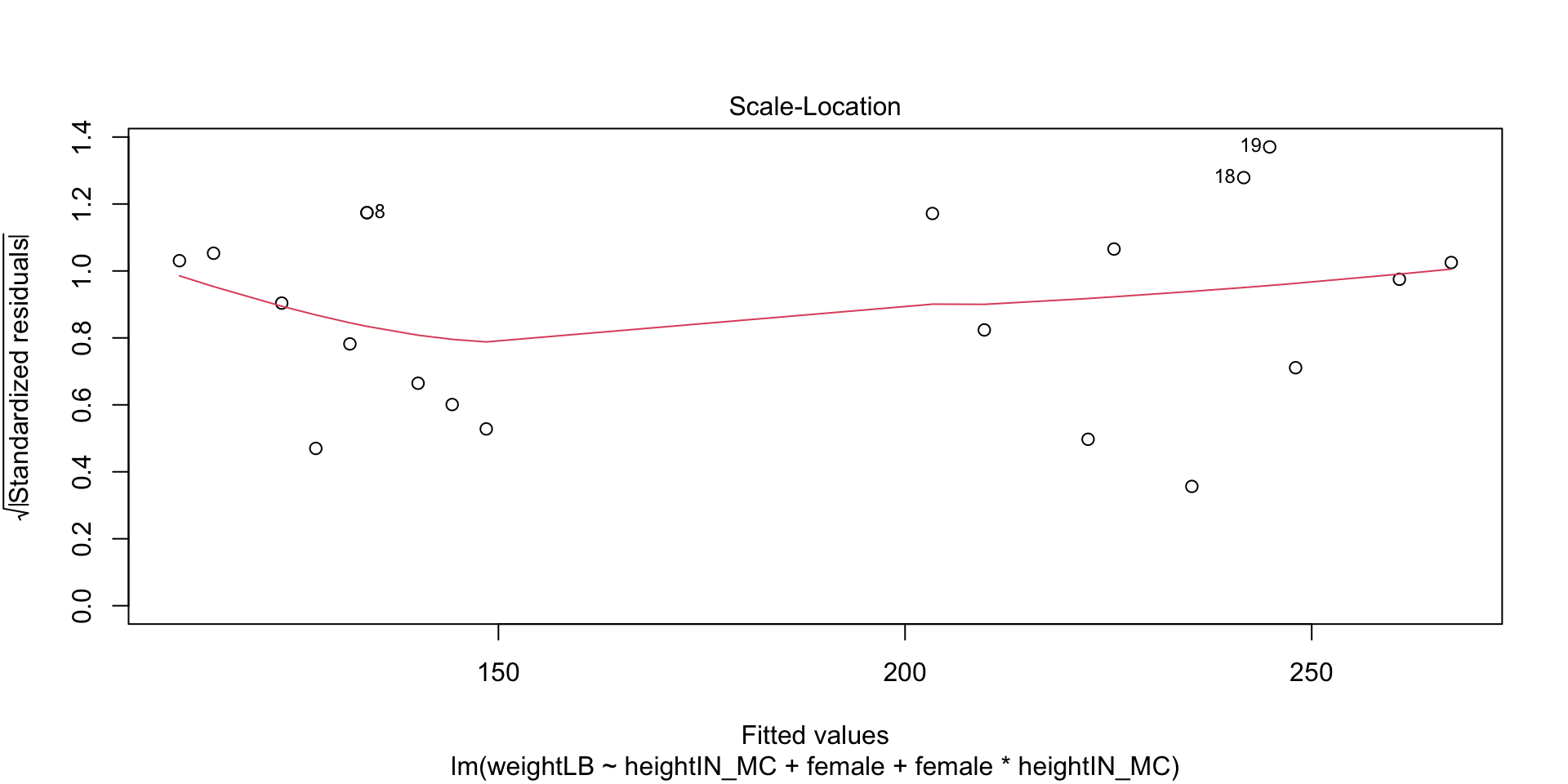
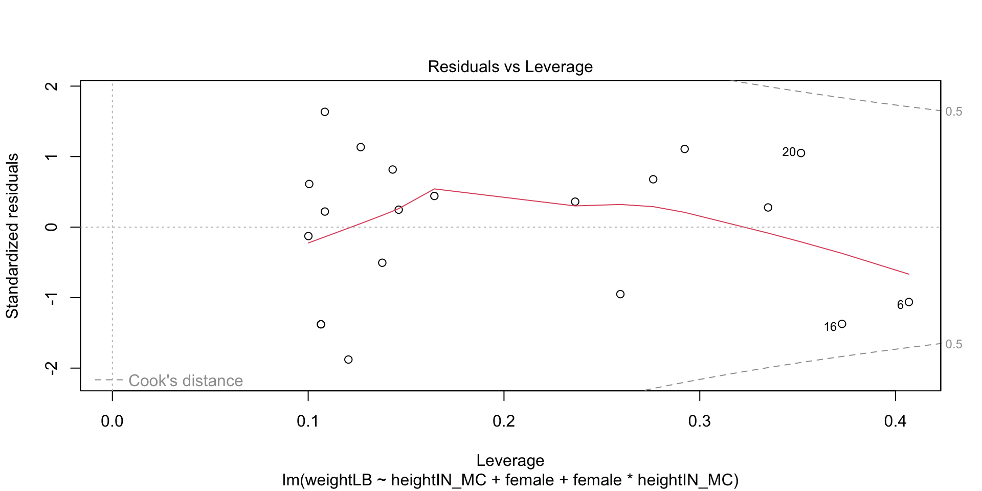
dat <- dataSexHeightWeight
dat$heightIN_MC <- dat$heightIN - mean(dat$heightIN)
dat$female <- dat$sex == 'F'
mod5 <- lm(weightLB ~ heightIN_MC + female + female*heightIN_MC, data = dat)
summary(mod5)

Call:
lm(formula = weightLB ~ heightIN_MC + female + female * heightIN_MC, 
    data = dat)

Residuals:
    Min      1Q  Median      3Q     Max 
-3.8312 -1.7797  0.4958  1.3575  3.3585 

Coefficients:
                       Estimate Std. Error t value Pr(>|t|)    
(Intercept)            222.1842     0.8381  265.11  < 2e-16 ***
heightIN_MC              3.1897     0.1114   28.65 3.55e-15 ***
femaleTRUE             -82.2719     1.2111  -67.93  < 2e-16 ***
heightIN_MC:femaleTRUE  -1.0939     0.1678   -6.52 7.07e-06 ***
---
Signif. codes:  0 '***' 0.001 '**' 0.01 '*' 0.05 '.' 0.1 ' ' 1

Residual standard error: 2.175 on 16 degrees of freedom
Multiple R-squared:  0.9987,    Adjusted R-squared:  0.9985 
F-statistic:  4250 on 3 and 16 DF,  p-value: < 2.2e-16

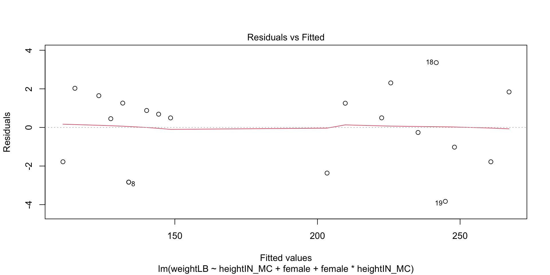
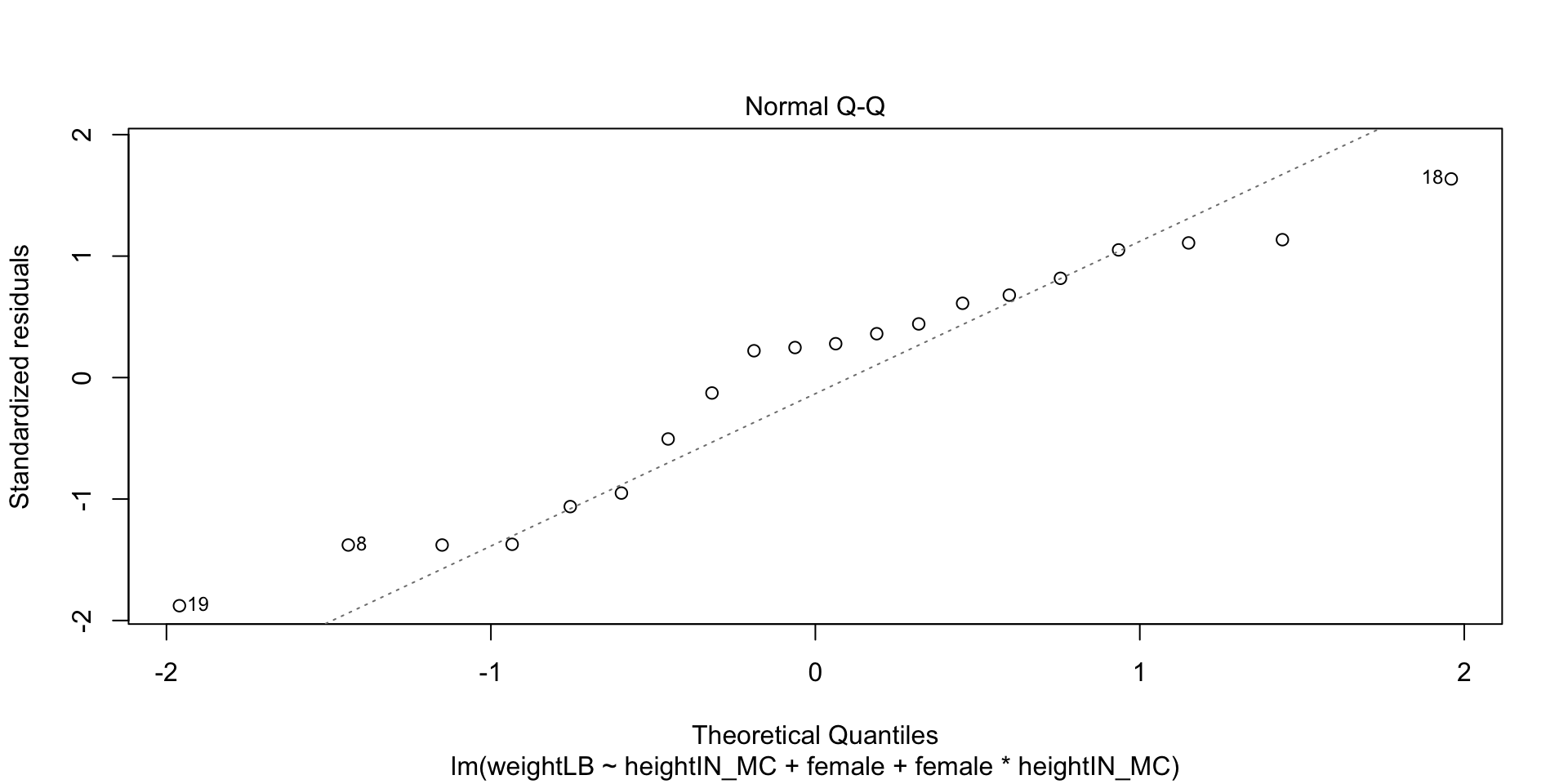
Picturing the GLM with Distributions

• The distributional assumptions of the GLM are the reason why we do not need to worry if our dependent variable is normally distributed

• Our dependent variable should be conditionally normal

• We can check this assumption by checking our assumption about the residuals, \(e_p \sim N(0, \sigma^2_e)\)

Assessing Distributional Assumptions Graphically

plot(mod5)

Hypothesis Tests for Normality

If a given test is significant, then it is saying that your data do not come from a normal distribution

In practice, test will give diverging information quite frequently: the best way to evaluate normality is to consider both plots and tests (approximate = good)

shapiro.test(mod5$residuals)

    Shapiro-Wilk normality test

data:  mod5$residuals
W = 0.95055, p-value = 0.3756

Wrapping Up

• Today was an introduction to mathematical statistics as a way to understand the implications statistical models make about data

• Although many of these topics do not seem directly relevant, they help provide insights that untrained analysts may not easily attain