| id | SATV | SATM |
|---|---|---|
| 1 | 520 | 580 |
| 2 | 520 | 550 |
| 3 | 460 | 440 |
| 4 | 560 | 530 |
| 5 | 430 | 440 |
| 6 | 490 | 530 |
| id | SATV | SATM | |
|---|---|---|---|
| 995 | 995 | 570 | 560 |
| 996 | 996 | 480 | 420 |
| 997 | 997 | 430 | 330 |
| 998 | 998 | 560 | 540 |
| 999 | 999 | 470 | 410 |
| 1000 | 1000 | 540 | 660 |
Matrix Algebra in R
Educational Statistics and Research Methods (ESRM) Program*
University of Arkansas
2024-10-07
| id | SATV | SATM |
|---|---|---|
| 1 | 520 | 580 |
| 2 | 520 | 550 |
| 3 | 460 | 440 |
| 4 | 560 | 530 |
| 5 | 430 | 440 |
| 6 | 490 | 530 |
| id | SATV | SATM | |
|---|---|---|---|
| 995 | 995 | 570 | 560 |
| 996 | 996 | 480 | 420 |
| 997 | 997 | 430 | 330 |
| 998 | 998 | 560 | 540 |
| 999 | 999 | 470 | 410 |
| 1000 | 1000 | 540 | 660 |
Matrix operations are fundamental to all modern statistical software.
When you installed R, R also comes with required matrix algorithm library for you. Two popular are BLAS and LAPACK
Other optimized libraries include OpenBLAS, AtlasBLAS, GotoBLAS, Intel MKL
{bash}} Matrix products: default LAPACK: /Library/Frameworks/R.framework/Versions/4.2-arm64/Resources/lib/libRlapack.dylib
From the LAPACK website,
LAPACK is written in Fortran 90 and provides routines for solving systems of simultaneous linear equations, least-squares solutions of linear systems of equations, eigenvalue problems, and singular value problems.
LAPACK routines are written so that as much as possible of the computation is performed by calls to the Basic Linear Algebra Subprograms (BLAS).
A matrix (denote as capitalized X) is composed of a set of elements
matrix[rowIndex, columnIndex] to extract the element with the position of rowIndex and columnIndex[1] 3
[1] 5
[1] 3 4
[1] 1 3 5In statistics, we use \(x_{ij}\) to represent one element with the position of ith row and jth column. For a example matrix \(\mathbf{X}\) with the size of 1000 rows and 2 columns.
The first subscript is the index of the rows
The second subscript is the index of the columns
\[ \mathbf{X} = \begin{bmatrix} x_{11} & x_{12}\\ x_{21} & x_{22}\\ \dots & \dots \\ x_{1000, 1} & x_{1000,2} \end{bmatrix} \]
A scalar is just a single number
The name scalar is important: the number “scales” a vector – it can make a vector “longer” or “shorter”.
Scalars are typically written without boldface:
\[ x_{11} = 520 \]
Each element of a matrix is a scalar.
Matrices can be multiplied by scalar so that each elements are multiplied by this scalar
The transpose of a matrix is a reorganization of the matrix by switching the indices for the rows and columns
\[ \mathbf{X} = \begin{bmatrix} 520 & 580\\ 520 & 550\\ \vdots & \vdots\\ 540 & 660\\ \end{bmatrix} \]
\[ \mathbf{X}^T = \begin{bmatrix} 520 & 520 & \cdots & 540\\ 580 & 550 & \cdots & 660 \end{bmatrix} \]
An element \(x_{ij}\) in the original matrix \(\mathbf{X}\) is now \(x_{ij}\) in the transposed matrix \(\mathbf{X}^T\)
Transposes are used to align matrices for operations where the sizes of matrices matter (such as matrix multiplication)
Square Matrix: A square matrix has the same number of rows and columns
Diagonal Matrix: A diagonal matrix is a square matrix with non-zero diagonal elements (\(x_{ij}\neq0\) for \(i=j\)) and zeros on the off-diagonal elements (\(x_{ij} =0\) for \(i\neq j\)):
\[ \mathbf{A} = \begin{bmatrix} 2.758 & 0 & 0 \\ 0 & 1.643 & 0 \\ 0 & 0 & 0.879\\ \end{bmatrix} \]
Symmetric Matrix: A symmetric matrix is a square matrix where all elements are reflected across the diagonal (\(x_{ij} = x_{ji}\))
Addition of a set of vectors (all multiplied by scalars) is called a linear combination:
\[ \mathbb{y} = a_1x_1 + a_2x_2 + \cdots + a_kx_k \]
Here, \(\mathbb{y}\) is the linear combination
For all k vectors, the set of all possible linear combinations is called their span
Typically not thought of in most analyses – but when working with things that don’t exist (latent variables) becomes somewhat importnat
In Data, linear combinations happen frequently:
Linear models (i.e., Regression and ANOVA)
Principal components analysis
Question: Does generalized linear model contains linear combinations? True, link function + a linear combination.
An important concept in vector geometry is that of the inner product of two vectors
\[ \mathbf{a} \cdot \mathbf{b} = a_{11}b_{11}+a_{21}b_{21}+\cdots+ a_{N1}b_{N1} = \sum_{i=1}^N{a_{i1}b_{i1}} \]
     [,1]
[1,]    8
     [,1]
[1,]    8
This is formally equivalent to (but usually slightly faster than) the call
t(x) %*% y(crossprod) orx %*% t(y)(tcrossprod).
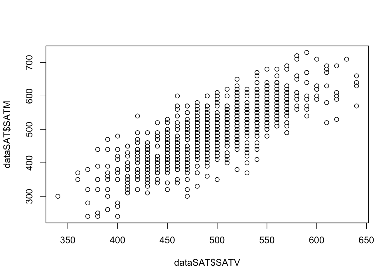
Using our example data dataSAT,
A matrix can be thought of as a collection of vectors
df$[name] or matrix[, index] to extract single vectorMatrix algebra defines a set of operations and entities on matrices
Definitions:
Identity matrix
Zero vector
Ones vector
Basic Operations:
Addition
Subtraction
Multiplication
“Division”
Matrix addition and subtraction are much like vector addition / subtraction
Rules: Matrices must be the same size (rows and columns)
Be careful!! R may not pop up error message when matrice + vector!
Method: the new matrix is constructed of element-by-element addition/subtraction of the previous matrices
Order: the order of the matrices (pre- and post-) does not matter
\[ \mathbf{A}_{(r \times c)} \mathbf{B}_{(c\times k)} = \mathbf{C}_{(r\times k)} \]
Rules: Pre-multiplying matrix must have number of columns equaling to the number of rows of the post-multiplying matrix
Method: the elements of the new matrix consist of the inner (dot) product of the row vectors of the pre-multiplying matrix and the column vectors of the post-multiplying matrix
Order: The order of the matrices matters
R: use %*% operator or crossprod to perform matrix multiplication
A = matrix(c(1, 2, 3, 4, 5, 6), nrow = 2, byrow = T)
B = matrix(c(5, 6, 7, 8, 9, 10), nrow = 3, byrow = T)
A
[,1] [,2] [,3]
[1,] 1 2 3
[2,] 4 5 6 [,1] [,2]
[1,] 5 6
[2,] 7 8
[3,] 9 10 [,1] [,2]
[1,] 46 52
[2,] 109 124 [,1] [,2] [,3]
[1,] 29 40 51
[2,] 39 54 69
[3,] 49 68 87The identity matrix (denoted as \(\mathbf{I}\)) is a matrix that pre- and post- multiplied by another matrix results in the original matrix:
\[ \mathbf{A}\mathbf{I} = \mathbf{A} \]
\[ \mathbf{I}\mathbf{A}=\mathbf{A} \]
The identity matrix is a square matrix that has:
Diagonal elements = 1
Off-diagonal elements = 0
\[ \mathbf{I}_{(3 \times 3)} = \begin{bmatrix} 1&0&0\\ 0&1&0\\ 0&0&1\\ \end{bmatrix} \]
R: we can create a identity matrix using diag
The zero and one vector is a column vector of zeros and ones:
\[ \mathbf{0}_{(3\times 1)} = \begin{bmatrix}0\\0\\0\end{bmatrix} \]
\[ \mathbf{1}_{(3\times 1)} = \begin{bmatrix}1\\1\\1\end{bmatrix} \]
When pre- or post- multiplied the matrix (\(\mathbf{A}\)) is the zero vector:
\[ \mathbf{A0=0} \]
\[ \mathbf{0^TA=0} \]
R:
Division from algebra:
First: \(\frac{a}{b} = b^{-1}a\)
Second: \(\frac{a}{b}=1\)
“Division” in matrices serves a similar role
For square symmetric matrices, an inverse matrix is a matrix that when pre- or post- multiplied with another matrix produces the identity matrix:
\[ \mathbf{A^{-1}A=I} \]
\[ \mathbf{AA^{-1}=I} \]
R: use solve() to calculate the matrix inverse
     [,1] [,2] [,3]
[1,]    1    0    0
[2,]    0    1    0
[3,] 0 0 1In data: the inverse shows up constantly in statistics
Using our SAT example
Our data matrix was size (\(1000\times 2\)), which is not invertible
However, \(\mathbf{X^TX}\) was size (\(2\times 2\)) – square and symmetric
          SATV      SATM
SATV 251797800 251928400
SATM 251928400 254862700\(\mathbf{(A+B)+C=A+(B+C)}\)
\(\mathbf{A+B=B+A}\)
\(c(\mathbf{A+B})=c\mathbf{A}+c\mathbf{B}\)
\((c+d)\mathbf{A} = c\mathbf{A} + d\mathbf{A}\)
\(\mathbf{(A+B)^T=A^T+B^T}\)
\((cd)\mathbf{A}=c(d\mathbf{A})\)
\((c\mathbf{A})^{T}=c\mathbf{A}^T\)
\(c\mathbf{(AB)} = (c\mathbf{A})\mathbf{B}\)
\(\mathbf{A(BC) = (AB)C}\)
We end our matrix discussion with some advanced topics
To help us throughout, let’s consider the correlation matrix of our SAT data:
          SATV      SATM
SATV 1.0000000 0.7752238
SATM 0.7752238 1.0000000
\[ R = \begin{bmatrix}1.00 & 0.78 \\ 0.78 & 1.00\end{bmatrix} \]
For a square matrix \(\mathbf{A}\) with p rows/columns, the matrix trace is the sum of the diagonal elements:
\[ tr\mathbf{A} = \sum_{i=1}^{p} a_{ii} \]
In R, we can use tr() in psych package to calculate matrix trace
For our data, the trace of the correlation matrix is 2
For all correlation matrices, the trace is equal to the number of variables
The trace is considered as the total variance in multivariate statistics
A square matrix can be characterized by a scalar value called a determinant:
\[ \text{det}\mathbf{A} =|\mathbf{A}| \]
Manual calculation of the determinant is tedious. In R, we use det() to calculate matrix determinant
The determinant is useful in statistics:
Shows up in multivariate statistical distributions
Is a measure of “generalized” variance of multiple variables
If the determinant is positive, the matrix is called positive definite \(\rightarrow\) the matrix has an inverse
If the determinant is not positive, the matrix is called non-positive definite \(\rightarrow\) the matrix does not have an inverse
Matrices show up nearly anytime multivariate statistics are used, often in the help/manual pages of the package you intend to use for analysis
You don’t have to do matrix algebra, but please do try to understand the concepts underlying matrices
Your working with multivariate statistics will be better off because of even a small amount of understanding
The covariance matrix \(\mathbf{S}\) is found by:
\[ \mathbf{S}=\frac{1}{N-1} \mathbf{(X-1\cdot\bar x^T)^T(X-1\cdot\bar x^T)} \]
\[ \mathbf{R = D^{-1}SD^{-1}} \] \[ \mathbf{S = DRD} \]
\[ \text{Generalized Sample Variance} = |\mathbf{S}| \]
It is a measure of spread across all variables
Reflecting how much overlapping area (covariance) across variables relative to the total variances occurs in the sample
Amount of overlap reduces the generalized sample variance
[1] 6527152# If no correlation
S_noCorr = S
S_noCorr[upper.tri(S_noCorr)] = S_noCorr[lower.tri(S_noCorr)] = 0
S_noCorr SATV SATM
SATV 2479.817 0.000
SATM 0.000 6596.303[1] 16357628[1] 0.399028# If correlation = 1
S_PerfCorr = S
S_PerfCorr[upper.tri(S_PerfCorr)] = S_PerfCorr[lower.tri(S_PerfCorr)] = prod(diag(S))
S_PerfCorr SATV SATM
SATV 2479.817 16357628.070
SATM 16357628.070 6596.303[1] -2.67572e+14The generalized sample variance is:
The total sample variance is the sum of the variances of each variable in the sample
\[ \text{Total Sample Variance} = \sum_{v=1}^{V} s^2_{x_i} = \text{tr}\mathbf{S} \]
Total sample variance for our SAT example:
The total sample variance does not take into consideration the covariances among the variables
\[ f(\mathbf{x}_p) = \frac{1}{(2\pi)^{\frac{V}2}|\mathbf{\Sigma}|^{\frac12}}\exp[-\frac{\color{tomato}{(x_p^T - \mu)^T \mathbf{\Sigma}^{-1}(x_p^T-\mu)}}{2}] \]
Where \(V\) represents number of variables and the highlighed is Mahalanobis Distance.
We use \(MVN(\mathbf{\mu, \Sigma})\) to represent a multivariate normal distribution with mean vector as \(\mathbf{\mu}\) and covariance matrix as \(\mathbf{\Sigma}\)
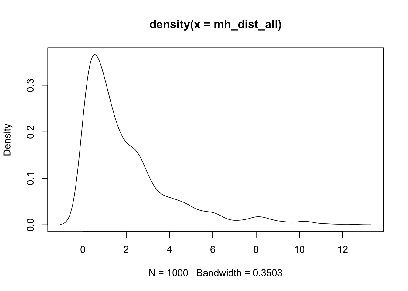
Similar to squared mean error in univariate distribution, we can calculate squared Mahalanobis Distance for each observable individual in the context of Multivariate Distribution
\[ d^2(x_p) = (x_p^T - \mu)^T \Sigma^{-1}(x_p^T-\mu) \]
mahalanobis followed by data vector (x), mean vector (center), and covariance matrix (cov) to calculate the squared Mahalanobis Distance for one individualSATV SATM
520 580 [1] 1.346228[1] 0.4211176[1] 0.6512687 [,1]
[1,] 1.346228The multivariate normal distribution has some useful properties that show up in statistical methods
If \(\mathbf{X}\) is distributed multivariate normally:
Similar to other distribution functions, we use dmvnorm to get the density given the observations and the parameters (mean vector and covariance matrix). rmvnorm can generate multiple samples given the distribution
  SATV   SATM
499.32 498.27 SATV SATM
SATV 2479.817 3135.359
SATM 3135.359 6596.303[1] 3.177814e-05[1] 5.046773e-05[1] -10682.62| SATV | SATM |
|---|---|
| 448.6690 | 346.5356 |
| 547.5522 | 623.7793 |
| 462.0201 | 405.1241 |
| 512.0536 | 500.8779 |
| 569.1587 | 504.6520 |
| 486.1675 | 474.9578 |
| 483.9587 | 490.9760 |
| 583.8711 | 677.7026 |
| 553.1567 | 628.5565 |
| 492.1799 | 501.6640 |
| 522.4085 | 580.9986 |
| 504.5034 | 524.3015 |
| 592.2830 | 643.1622 |
| 519.5650 | 556.0304 |
| 454.2103 | 498.6606 |
| 596.5938 | 690.5468 |
| 543.7172 | 605.6825 |
| 493.2891 | 530.0512 |
| 493.6388 | 476.8900 |
| 479.7672 | 495.8584 |
We are now ready to discuss multivariate models and the art/science of multivariate modeling
Many of the concepts of univariate models carry over
Matrix algebra was necessary so as to concisely talk about our distributions (which will soon be models)
The multivariate normal distribution will be necessary to understand as it is the most commonly used distribution for estimation of multivariate models
Next class we will get back into data analysis – but for multivariate observations…using R’s lavaan package for path analysis
![]()
ESRM 64503 - Lecture 07: Matrix Algebra