──────────────────────────────────────────────────────────────────────────────
Describe dataMath[, 2:8] (data.frame):
data frame: 350 obs. of 7 variables
145 complete cases (41.4%)
Nr Class ColName NAs Levels
1 int hsl 36 (10.3%)
2 int cc 37 (10.6%)
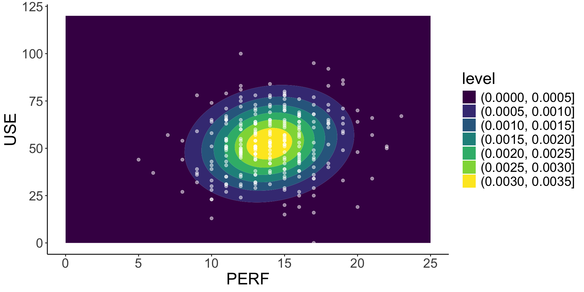
3 int use 24 (6.9%)
4 int msc 39 (11.1%)
5 int mas 46 (13.1%)
6 int mse 34 (9.7%)
7 int perf 60 (17.1%)
──────────────────────────────────────────────────────────────────────────────
1 - hsl (integer)
length n NAs unique 0s mean meanCI'
350 314 36 8 0 4.92 4.92
89.7% 10.3% 0.0% 4.92
.05 .10 .25 median .75 .90 .95
3.00 3.00 4.00 5.00 6.00 6.00 7.00
range sd vcoef mad IQR skew kurt
7.00 1.32 0.27 1.48 2.00 -0.26 -0.41
value freq perc cumfreq cumperc
1 1 1 0.3% 1 0.3%
2 2 11 3.5% 12 3.8%
3 3 34 10.8% 46 14.6%
4 4 71 22.6% 117 37.3%
5 5 79 25.2% 196 62.4%
6 6 88 28.0% 284 90.4%
7 7 27 8.6% 311 99.0%
8 8 3 1.0% 314 100.0%
' 0%-CI (classic)
──────────────────────────────────────────────────────────────────────────────
2 - cc (integer)
length n NAs unique 0s mean meanCI'
350 313 37 28 21 10.31 10.31
89.4% 10.6% 6.0% 10.31
.05 .10 .25 median .75 .90 .95
0.00 2.00 6.00 10.00 14.00 19.00 20.00
range sd vcoef mad IQR skew kurt
27.00 5.89 0.57 5.93 8.00 0.17 -0.43
lowest : 0 (21), 1 (5), 2 (9), 3 (9), 4 (12)
highest: 23, 24, 25, 26, 27
heap(?): remarkable frequency (8.6%) for the mode(s) (= 10, 13)
' 0%-CI (classic)
──────────────────────────────────────────────────────────────────────────────
3 - use (integer)
length n NAs unique 0s mean meanCI'
350 326 24 71 1 52.50 52.50
93.1% 6.9% 0.3% 52.50
.05 .10 .25 median .75 .90 .95
25.50 31.00 42.25 52.00 64.00 71.50 77.75
range sd vcoef mad IQR skew kurt
100.00 15.81 0.30 16.31 21.75 -0.11 -0.08
lowest : 0, 13, 15, 16, 19 (2)
highest: 84 (2), 86, 92, 95, 100
' 0%-CI (classic)
──────────────────────────────────────────────────────────────────────────────
4 - msc (integer)
length n NAs unique 0s mean meanCI'
350 311 39 76 0 49.79 49.79
88.9% 11.1% 0.0% 49.79
.05 .10 .25 median .75 .90 .95
24.00 29.00 38.00 49.00 61.00 72.00 80.50
range sd vcoef mad IQR skew kurt
98.00 16.96 0.34 16.31 23.00 0.23 -0.09
lowest : 5, 9, 12, 15, 16 (2)
highest: 87 (3), 89, 91, 94, 103
' 0%-CI (classic)
──────────────────────────────────────────────────────────────────────────────
5 - mas (integer)
length n NAs unique 0s mean meanCI'
350 304 46 57 1 31.50 31.50
86.9% 13.1% 0.3% 31.50
.05 .10 .25 median .75 .90 .95
13.00 17.00 24.75 32.00 39.00 45.70 50.00
range sd vcoef mad IQR skew kurt
62.00 11.32 0.36 10.38 14.25 -0.13 -0.17
lowest : 0, 2, 3 (2), 5, 6
highest: 54 (2), 55 (2), 56, 58, 62
' 0%-CI (classic)
──────────────────────────────────────────────────────────────────────────────
6 - mse (integer)
length n NAs unique 0s mean meanCI'
350 316 34 56 0 73.41 73.41
90.3% 9.7% 0.0% 73.41
.05 .10 .25 median .75 .90 .95
54.00 58.00 65.00 73.00 81.00 88.50 92.25
range sd vcoef mad IQR skew kurt
60.00 11.89 0.16 11.86 16.00 0.06 -0.26
lowest : 45 (2), 46, 47, 49 (2), 50 (4)
highest: 98, 100, 101 (2), 103, 105 (2)
' 0%-CI (classic)
──────────────────────────────────────────────────────────────────────────────
7 - perf (integer)
length n NAs unique 0s mean meanCI'
350 290 60 19 0 13.97 13.97
82.9% 17.1% 0.0% 13.97
.05 .10 .25 median .75 .90 .95
9.45 10.00 12.00 14.00 16.00 18.00 19.00
range sd vcoef mad IQR skew kurt
18.00 2.96 0.21 2.97 4.00 0.16 0.14
lowest : 5, 6, 7 (2), 8 (3), 9 (8)
highest: 19 (10), 20 (4), 21 (3), 22 (2), 23
heap(?): remarkable frequency (13.8%) for the mode(s) (= 13)
' 0%-CI (classic)