library(animation)
library(gganimate)
library(ggplot2)
library(tidyverse)
library(knitr)
library(here)2018-2022年教育期刊的引用数可视化
教程
(2019’s Summary) 简单的描述一下,和教育相关的意外只有Review of Educational Research。还有令我意外的是,Journal of Mixed Methods Research也有上榜,看来纯方法的期刊也可以拥有超高应用数。原因之一大概是mixed method在社会科学的统治地位。总的来说,霸榜最久的是MMWR (Morbidity and mortality weekly report)以及National vital statistics reports。另外,用R做gif果然帧数不够,真要像油管那样的话得转成mp4格式才行。
Code
tidize <- function(data) {
  dat.tidy <- dat %>%
    select(Title, Ref....Doc.) %>% # average amount of references per document
    rename(Citation = Ref....Doc.) %>%
    mutate(
      Citation = as.numeric(gsub(",", "", .$Citation)),
      rank = rank(-Citation)) %>%
    arrange(desc(Citation)) %>%
    .[1:10,]
  return(dat.tidy)
}
root_dir <- "postsCN/2019-12-31-animation"
filenames <- list.files(here(root_dir), pattern = '.csv')
years <- as.numeric(unlist(regmatches(filenames, gregexpr("[[:digit:]]+", filenames))))
dat.list <- list()
length(dat.list) <- length(filenames)
# dat <- read.csv(here(root_dir, filenames[1]), header = TRUE, sep = ";", check.names = T, stringsAsFactors = FALSE)
# colnames(dat)
for (n in seq_along(filenames)) {
dat <- read.csv(here(root_dir, filenames[n]), header = TRUE, sep = ";", check.names = T, stringsAsFactors = FALSE)
dat = tidize(dat)
dat$Year = years[n]
dat.list[[n]] <- dat
}
dat.comb <- do.call("rbind", dat.list)
dat.comb$Year <- factor(dat.comb$Year, levels = years)
dat.comb$Title <- factor(dat.comb$Title)staticplot <-
ggplot(dat.comb,
aes(x = rank, group = Year, fill = as.factor(Title), color = as.factor(Title))) +
geom_tile(aes(y = Citation/2,
height = Citation,
width = 0.8), alpha = 0.1) +
geom_text(aes(y = 3000, label = paste(" ",Title)), hjust = 0, color = "black") +
geom_text(aes(y= Citation + 20,label = Citation, hjust= 0)) + # the number
guides(color = FALSE, fill = FALSE) +
coord_flip(clip = "off", expand = FALSE) +
scale_y_continuous(labels = scales::comma, limits = c(0, 25000)) +
scale_x_reverse(breaks = 1:20) +
labs(y = "Citation") +
theme(
axis.title.x=element_blank(),
axis.ticks.x=element_blank(),
axis.text.x=element_blank(),
axis.title.y=element_blank(),
axis.text.y= element_blank(),
axis.ticks.y=element_blank()) +
theme_classic()
staticplot + facet_wrap(~ Year, ncol = 1)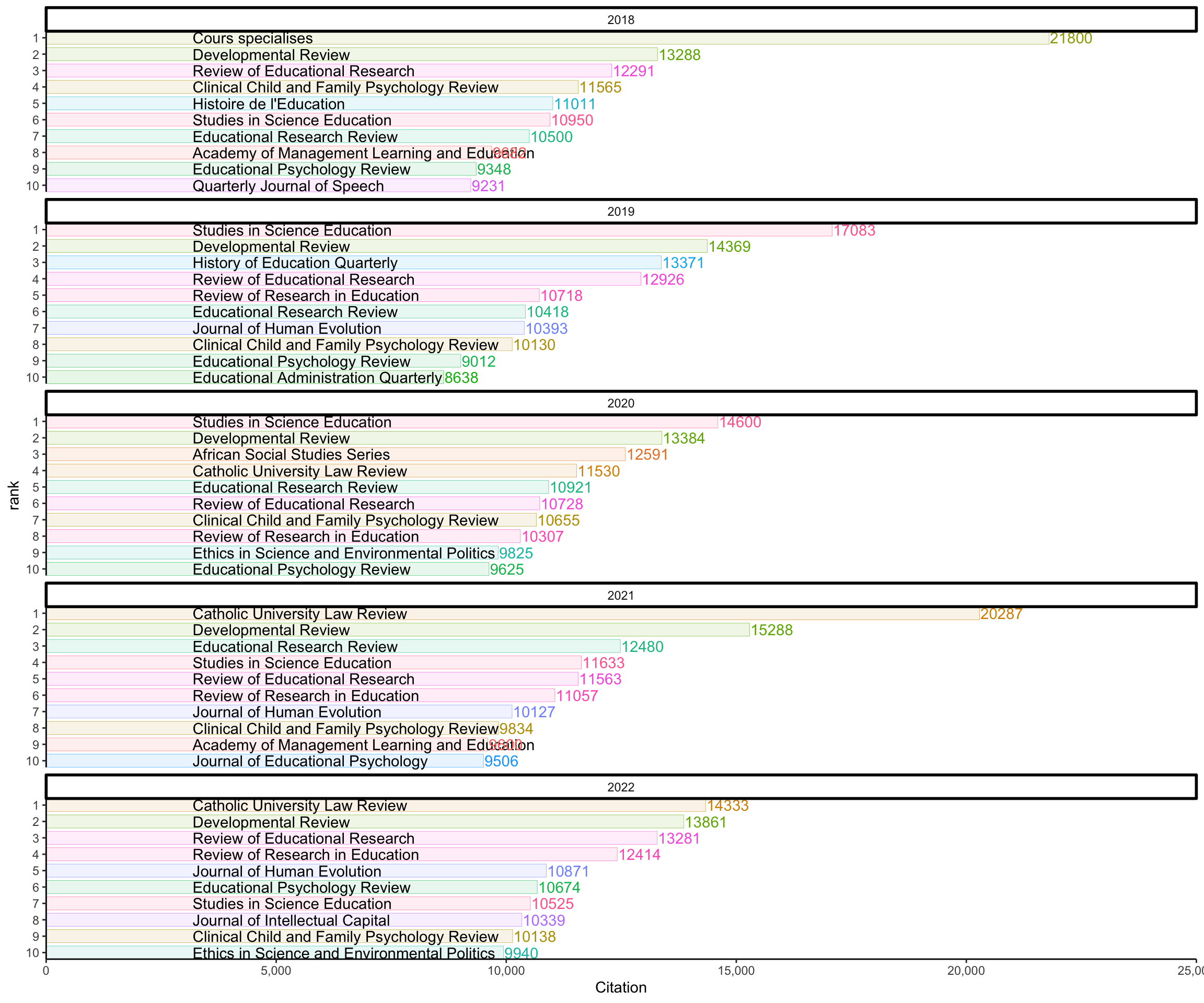
(anim =
    staticplot +
    transition_states(Year, transition_length = 20, state_length = 1) +
    view_follow(fixed_y = TRUE, fixed_x = T) +
    labs(
      #title = 'Year: {closest_state}',
      caption = "Author: Jihong Zhang",
      render = gifski_renderer()
    ))
Original R Code
#setwd("~/Desktop/impact_factor/")
filenames <- list.files("~/Desktop/impact_factor/")
years <- as.numeric(unlist(regmatches(filenames, gregexpr("[[:digit:]]+", filenames))))

dat.list <- list()
length(dat.list) <- length(filenames)

for (n in seq_along(filenames)) {
  dat <- read.csv(paste0("~/Desktop/impact_factor/", filenames[n]), header = TRUE, sep = ";", check.names = T, stringsAsFactors = FALSE)
  dat = tidize(dat)
  dat$year = years[n]
  dat.list[[n]] <- dat
}
dat.comb <- do.call("rbind", dat.list)

dat.comb[dat.comb$Title == "MMWR. Recommendations and reports : Morbidity and mortality weekly report. Recommendations and reports / Centers for Disease Control", "Title"] = "MMWR:Recommendations and reports"
dat.comb[dat.comb$Title == "National vital statistics reports : from the Centers for Disease Control and Prevention, National Center for Health Statistics, National Vital Statistics System", "Title"] = "National vital statistics reports"
dat.comb[dat.comb$Title == "MMWR. Surveillance summaries : Morbidity and mortality weekly report. Surveillance summaries / CDC", "Title"] = "MMWR:Surveillance summaries"
dat.comb[dat.comb$Title == "Energy Education Science and Technology Part B: Social and Educational Studies", "Title"] = "Energy Education Science and Technology"

staticplot <- ggplot(dat.comb, aes(x = (rank), group = Title,
       fill = as.factor(Title), color = as.factor(Title))) +
  geom_tile(aes(y = Citation/2,
                height = Citation,
                width = 1), alpha = 0.8) +
  geom_text(aes(y = 3000, label = paste(" ",Title)), hjust = 0, color = "black") +
  geom_text(aes(y= Citation + 20,label = Citation, hjust= 0)) + # the number
  guides(color = FALSE, fill = FALSE) +
  coord_flip(clip = "off", expand = FALSE) +
  scale_y_continuous(labels = scales::comma) +
  scale_x_reverse() +
  theme(
    axis.title.x=element_blank(),
    axis.ticks.x=element_blank(),
    axis.text.x=element_blank(),
    axis.title.y=element_blank(),
    axis.text.y= element_blank(),
    axis.ticks.y=element_blank())

(anim = staticplot +
  transition_states(year, transition_length = 10, state_length = 1) +
  view_follow(fixed_y = TRUE) +
  labs(title = 'Citations of The year: {closest_state}',
       subtitle  =  "Top 10 Journals in Social Sciences",
caption = "Author: Jihong Zhang"))animate(anim, renderer = gifski_renderer("/Users/jzhang285/Documents/Projects/hugo-academic-jihong/static/img/citation_journals.gif"))sources: https://www.scimagojr.com/journalrank.php?category=3304&min=0&min_type=cd