Lecture 01
Course and Bayesian Analysis Introduction
Educational Statistics and Research Methods
Today’s Lecture Objectives
- Introduction to Bayesian Analysis
but, before we begin…
Background: What is Bayesian?
Where does the word “Bayesian” come from?
The term “Bayesian” is named after Thomas Bayes (1701-1761), an English statistician. He developed a mathematical theorem that describes how to update probabilities based on new evidence. His work was published posthumously in 1763 and has since become the foundation of Bayesian statistics.
- How to Pronounce Bayesian (Real Life Examples!)
- “B-Asian” or “Bayes-ian”?
- What does “Bayesian” mean? Assign probabilities to everything!
- Frequentist vs Bayesian
- Example: In the U.S., are there more male or female Asian faculty?
- Frequentist: If “Male:Female = 1:1 out of Asian Faculty” is fixed, how is the probability that the data happens?
- Bayesian: If I believe Male:Female = 1:2 but the data says 1:1, to what degree do I need to update my belief?
- Example: In the U.S., are there more male or female Asian faculty?
Bayesian Model Components
Simple Definition: Bayesian statistics is a method that combines what we already know (prior knowledge) with new evidence (data) to update our beliefs about uncertain things. Everything is treated as having some level of uncertainty that can be expressed as a probability.
- What we see: Observed Data (the data you actually collect)
- What we cannot see: Future Data, Data yet to be collected, Parameters, Population Distribution
Take home Note: Everything is random in Bayesian
- Observed Data: Some random information given a unknown generation process
- Parameter: The random components controlling the generation process
Take home Note: Every random component can be expressed as probability!
- The probability of observed data given parameters: \(p(\text{Observed Data}|\text{Parameters})\) = Data Likelihood
- The probability of parameters: \(p(\text{Parameters})\) = Prior Distribution
- The probability of parameters given observed data: \(p(\text{Parameters}|\text{Observed Data})\) = Posterior Distribution*
Bayesian Logic
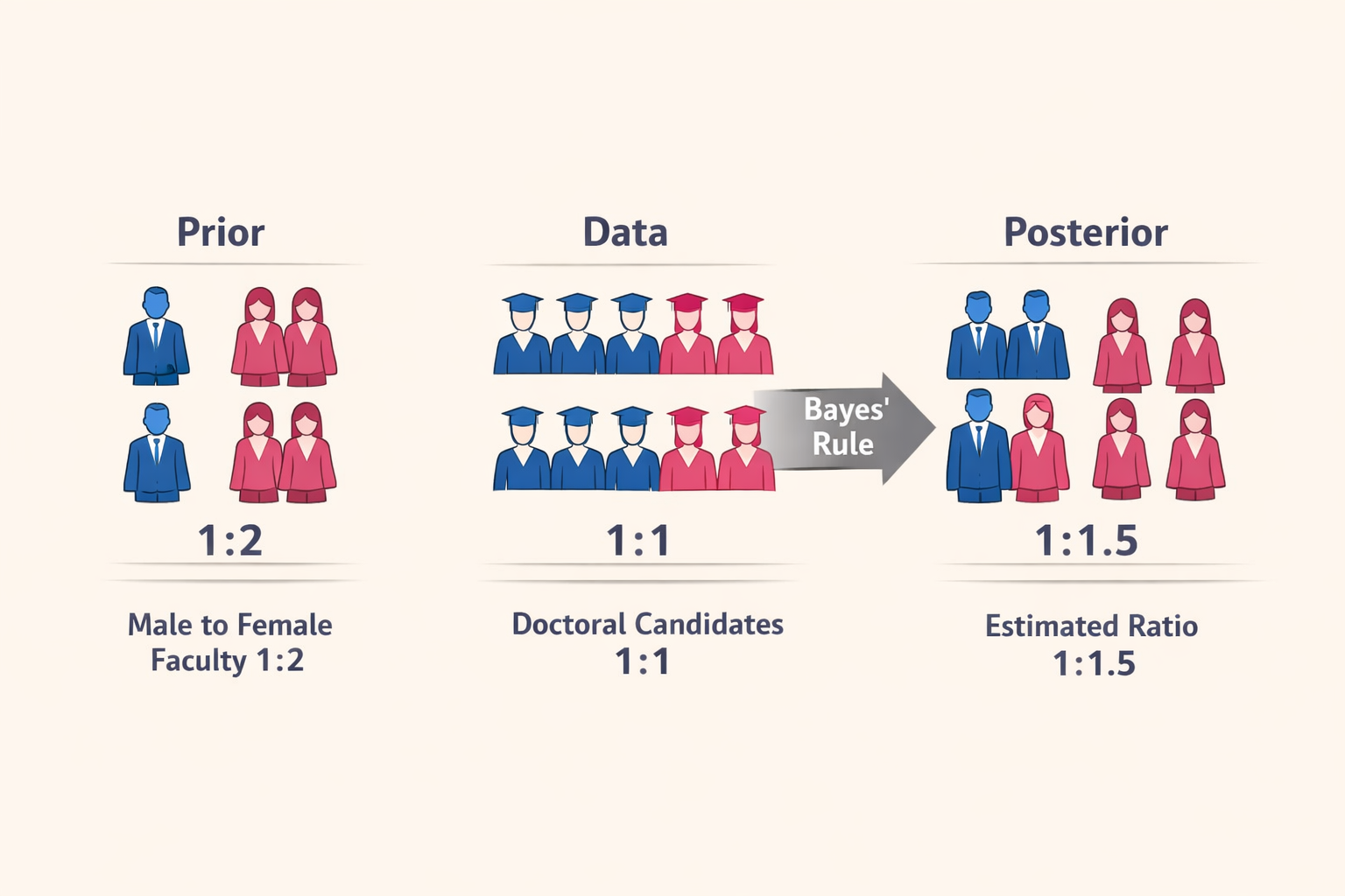
A toy example:
The ratio of male Asian faculty to female Asian faculty is about 1:2 (Prior). We obtained information from 2000 doctoral candidates suggesting the gender ratio is 1:1 (Data; Likelihood given the true ratio we don’t know). Based on Bayes’ rule, the estimate for the ratio is probably 1:1.5 (Posterior) after combining these two statements.
Bayesian Analysis: Why It Is Used?
There are at least four main reasons why people use Bayesian Analysis:
- Missing data
- Multiple imputation (fill in missing data points with external information)
- More complicated model for certain types of missing data
- Lack of software capable of handling large-sized analyses
- Have a zero-inflated Poisson model with 1000 observations and 1000 parameters? No problem in Bayesian!
Bayesian Analysis: Why It Is Used? (Cont.)
- New complex models not available in frequentist framework
- Have a new model? (A model that estimates the probability students choose the right answers then choose the wrong answers in a multiple choice test?)
- Enjoy the Bayesian thinking process
- It is a way of thinking that everything is random and everything can be expressed as probability. It is a way of thinking that we can update our belief as we collect more data. It is a way of thinking that we can use our prior knowledge to help us understand the data.
Bayesian Analysis: Why It Is Used? (Cont.)
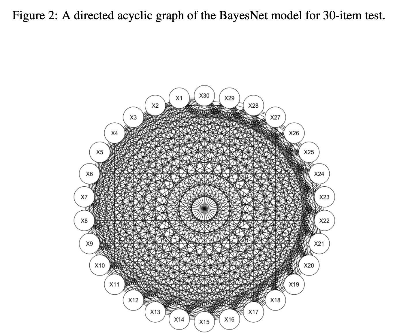
I created a BayesNet model for 30 survey items. It simulates the complete item relationships, which can still be estimated using Bayesian analysis.
Bayesian Analysis: Issues
- Subjective vs. Objective
- Prior distribution is subjective. It is based on your prior knowledge.
- However, 1) Scientific judgement is always subjective 2) you can use objective prior distribution to avoid this issue.
- Computationally Intensive
- It is not a problem anymore. We have computers.
- But we still need weeks or months to get results for some complex models and large datasets
- Difficult to understand
Bayesian Analysis is popular
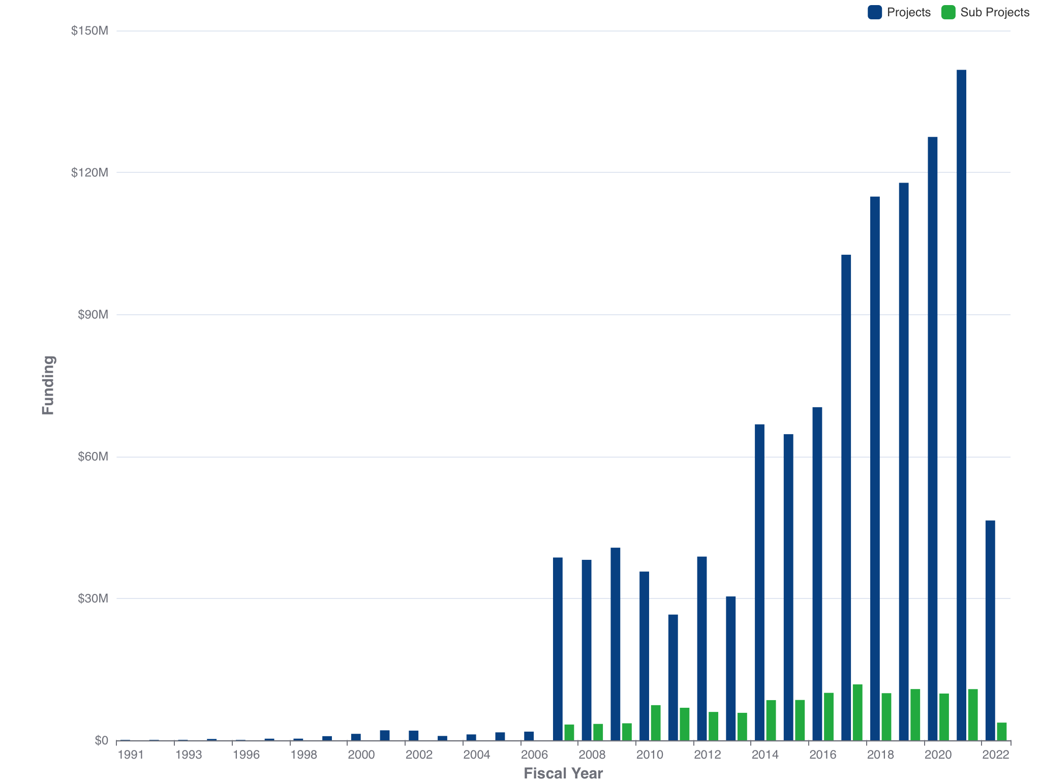
Funding available only for NIH, CDC, FDA, AHRQ, and ACF 2020 Spring. Source: https://report.nih.gov/
What topics Bayesian Analysis can cover?
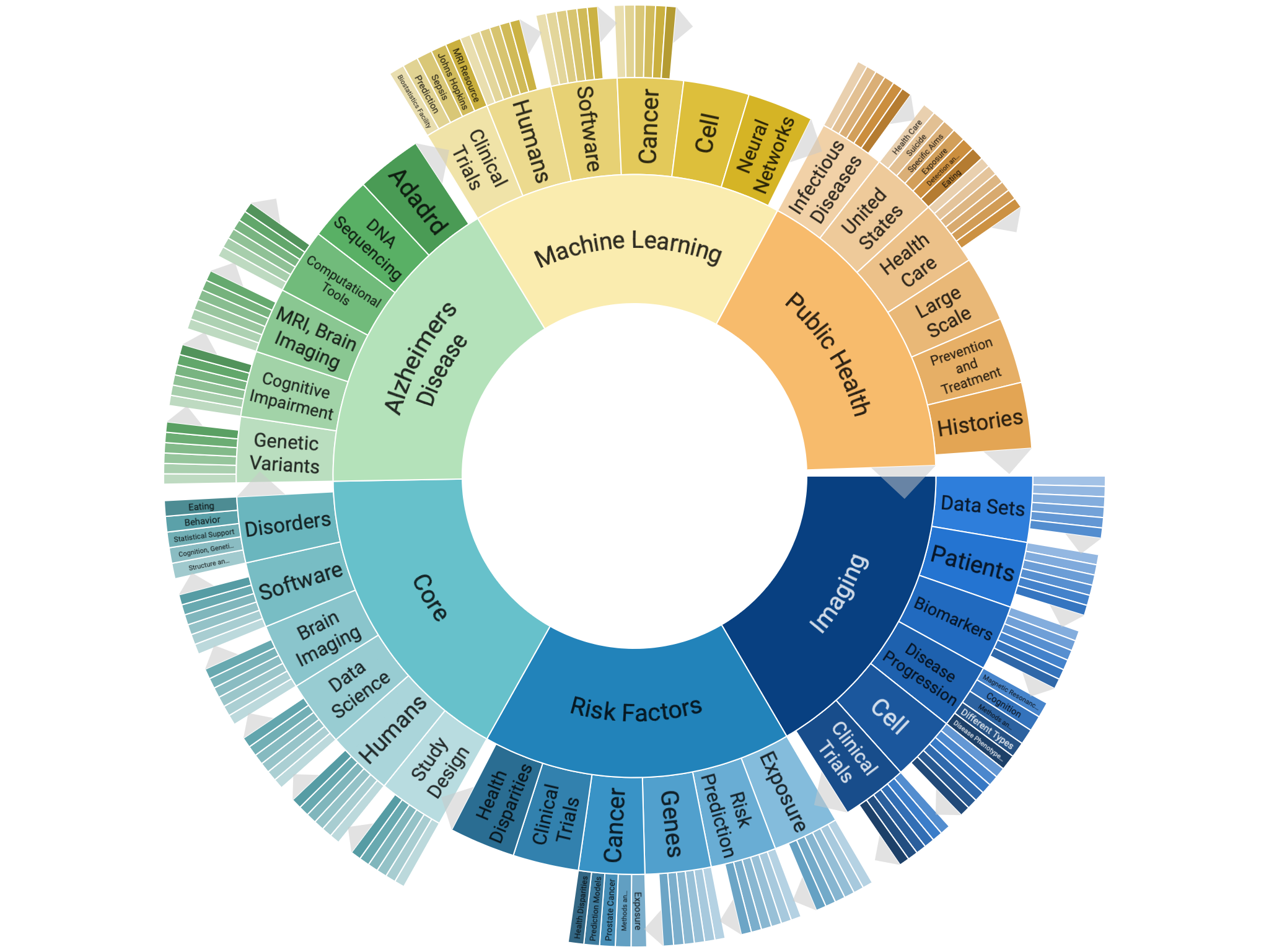
Funding available only for NIH, CDC, FDA, AHRQ, and ACF 2020 Spring. Source: https://report.nih.gov/
Case Study: Medical Test Example
The Scenario
Suppose you are a doctor and a patient comes in for a rare disease screening:
The disease affects 1% of the population (Prior Information)
You have a diagnostic test that:
- Correctly identifies 95% of people who have the disease (Sensitivity)
- Correctly identifies 90% of people who don’t have the disease (Specificity)
Question: If a patient tests positive, what is the probability they actually have the disease?
Case Study: Understanding the Test
Confusion Matrix (Test Characteristics)
| Test Positive | Test Negative | |
|---|---|---|
| Has Disease | True Positive = 95% | False Negative = 5% |
| (Correctly detected) | (Missed cases) | |
| No Disease | False Positive = 10% | True Negative = 90% |
| (False alarm) | (Correctly ruled out) |
Key Terms:
- Sensitivity = True Positive Rate = 95%
- Specificity = True Negative Rate = 90%
Case Study: Setting Up the Problem
What We Know (Define Our Probabilities):
Prior Distribution: \(P(\text{Disease}) = 0.01\) and \(P(\text{No Disease}) = 0.99\)
Likelihood: The probability of test results given disease status
- \(P(\text{Positive Test}|\text{Disease}) = 0.95\) (true positive)
- \(P(\text{Positive Test}|\text{No Disease}) = 0.10\) (false positive)
What We Want: Posterior Distribution
- \(P(\text{Disease}|\text{Positive Test}) = ?\)
Question: Can you guess how large is this probability?
Case Study: Applying Bayes’ Rule
\[P(\text{Disease}|\text{Positive Test}) = \frac{P(\text{Positive Test}|\text{Disease}) \times P(\text{Disease})}{P(\text{Positive Test})}\]
We need to find \(P(\text{Positive Test})\) first (total probability of testing positive):
\[P(\text{Positive Test}) = P(\text{Positive}|\text{Disease}) \times P(\text{Disease})\] \[+ P(\text{Positive}|\text{No Disease}) \times P(\text{No Disease})\]
\[= 0.95 \times 0.01 + 0.10 \times 0.99 = 0.0095 + 0.099 = 0.1085\]
Case Study: The Calculation
Now we can calculate the posterior:
\[P(\text{Disease}|\text{Positive Test}) = \frac{0.95 \times 0.01}{0.1085} = \frac{0.0095}{0.1085} \approx 0.0876\]
Result: Only about 8.76% chance the patient actually has the disease!
Case Study: Interpretation
Why Is the Probability So Low?
- Prior matters: The disease is rare (1%), so most people don’t have it
- False positives: 10% false positive rate means many healthy people test positive
- Bayesian updating: We updated our belief from 1% (prior) to 8.76% (posterior)
Key Insight:
- Out of 10,000 people:
- 100 have the disease (1%); 95 test positive ✓
- 9,900 are healthy (99%); 990 test positive (false alarm!)
- Total positive tests: 95 + 990 = 1,085
- Probability of disease given positive: \(\frac{95}{1,085} \approx 8.76\%\)
Case Study: What If We Test Again?
Second Test After First Positive:
New Prior: Our posterior becomes the new prior = P(Disease)’ = 0.0876 (8.76%)
If the second test is also positive:
\[P(\text{Disease}|\text{2nd Positive}) = \frac{0.95 \times 0.0876}{0.95 \times 0.0876 + 0.10 \times 0.9124}\]
\[= \frac{0.0832}{0.0832 + 0.0912} \approx 0.477\]
Result: Now about 47.7% chance of the individual actually having disease! This is sequential Bayesian updating.
Case Study: Take-Home Messages
- Prior information is powerful: The 1% base rate strongly influences the result
- Bayesian updating is iterative: We can keep updating as new data arrives
- Counterintuitive results: A “95% accurate” test doesn’t mean 95% chance of disease
- Everything is probability: Disease status, test results, all expressed as probabilities
This is the essence of Bayesian thinking: combining prior knowledge with data to update beliefs!
Wrapping Up
- We understand what “Bayesian” means and its components.
- How Bayesian estimation differs from other estimation methods, such as maximum likelihood
- We also know that Bayesian analysis is popular in many fields, especially for complex data
Next Class
We will talk about how Bayesian methods works in a little bit more technical way.
Suggestions
Your opinions are very important to me. Feel free to let me know if you have any suggestions on the course.