library(tidyr)
library(dplyr)
library(ggplot2)
rate_list = seq(0.1, 1, 0.2)
pdf_points = sapply(rate_list, \(x) dexp(seq(0, 20, 0.01), x)) |> as.data.frame()
colnames(pdf_points) <- rate_list
pdf_points$x = seq(0, 20, 0.01)
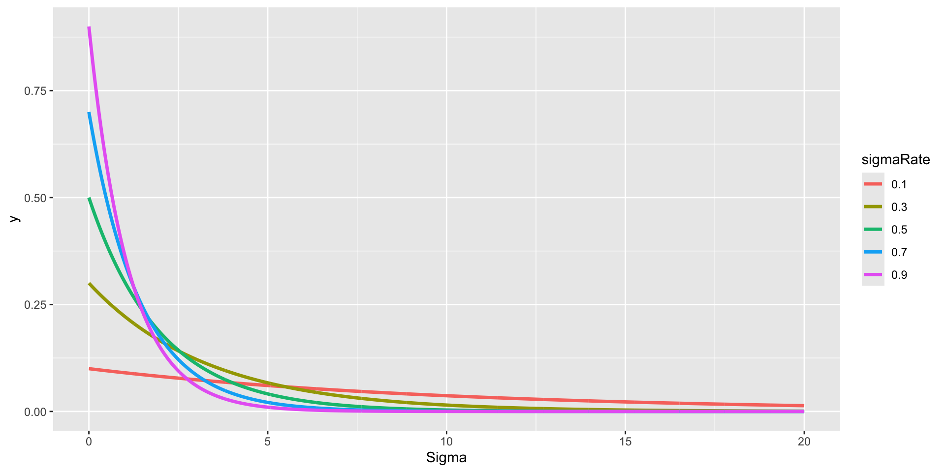
pdf_points %>%
pivot_longer(-x, values_to = 'y') %>%
mutate(
sigmaRate = factor(name, levels = rate_list)
) %>%
ggplot() +
geom_path(aes(x = x, y = y, color = sigmaRate, group = sigmaRate), size = 1.2) +
scale_x_continuous(limits = c(0, 20)) +
labs(x = "Sigma")library(tidyr)
library(dplyr)
library(ggplot2)
rate_list = seq(0.1, 1, 0.2)
pdf_points = sapply(rate_list, \(x) dexp(seq(0, 20, 0.01), x)) |> as.data.frame()
colnames(pdf_points) <- rate_list
pdf_points$x = seq(0, 20, 0.01)
pdf_points %>%
pivot_longer(-x, values_to = 'y') %>%
mutate(
sigmaRate = factor(name, levels = rate_list)
) %>%
ggplot() +
geom_path(aes(x = x, y = y, color = sigmaRate, group = sigmaRate), size = 1.2) +
scale_x_continuous(limits = c(0, 20)) +
labs(x = "Sigma")