Lecture 07

Generalized Measurement Models: Modeling Observed Data

Jihong Zhang

Educational Statistics and Research Methods

Previous Class

1. We used two simulation data sets to introduce how Stan can be used for factor analysis

• A simple structure
• A structure with cross-loading

2. What we left is how to interpret parameters in factor analysis
3. We also need to refresh our memory of R coding and Stan coding we’ve learnt so far

Today’s Lecture Objectives

1. Quickly go through our R code file so far
2. Show different modeling specifications for different types of item response data
3. Show how parameterization differs for standardized latent variables vs. marker item scale identification

Example Data: Conspiracy Theories

• Today’s example is from a bootstrap resample of 177 undergraduate students at a large state university in the Midwest.

• The survey was a measure of 10 questions about their beliefs in various conspiracy theories that were being passed around the internet in the early 2010s

• All item responses were on a 5-point Likert scale with:

  • Strong Disagree

  • Disagree

  • Neither Agree nor Disagree

  • Agree

  • Strongly Agree

• The purpose of this survey was to study individual beliefs regarding conspiracies.

• Our purpose in using this instrument is to provide a context that we all may find relevant as many of these conspiracies are still prevalent.

Conspiracy Theory Q1-Q5¹

1. The U.S. invasion of Iraq was not part of a campaign to fight terrorism, but was driven by oil companies and Jews in the U.S. and Israel.
2. Certain U.S. government officials planned the attacks of September 11, 2001 because they wanted the United States to go to war in the Middle East.
3. President Barack Obama was not really born in the United States and does not have an authentic Hawaiian birth certificate.
4. The current financial crisis was secretly orchestrated by a small group of Wall Street bankers to extend the power of the Federal Reserve and further their control of the world’s economy.
5. Vapor trails left by aircraft are actually chemical agents deliberately sprayed in a clandestine program directed by government officials.

1. Built by Dr. Jonathan Templin

Conspiracy Theory Q6-Q10

1. Billionaire George Soros is behind a hidden plot to destabilize the American government, take control of the media, and put the world under his control.

2. The U.S. government is mandating the switch to compact fluorescent light bulbs because such lights make people more obedient and easier to control.

3. Government officials are covertly Building a 12-lane “NAFTA superhighway” that runs from Mexico to Canada through America’s heartland.

4. Government officials purposely developed and spread drugs like crack-cocaine and diseases like AIDS in order to destroy the African American community.

5. God sent Hurricane Katrina to punish America for its sins.

Response Distribution

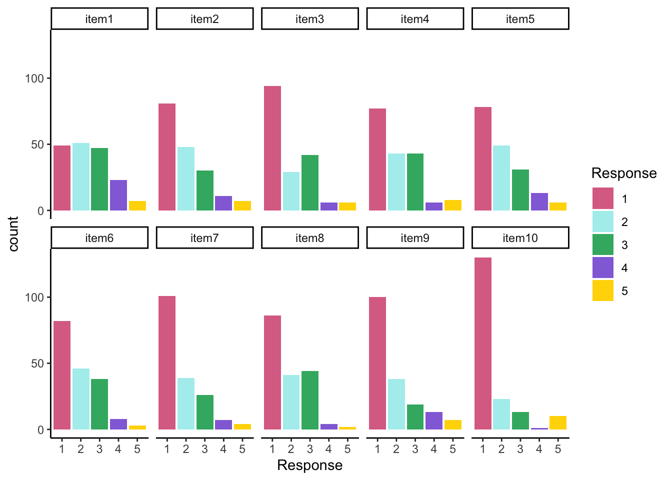
All items seem to be positive skewed

## ── Attaching core tidyverse packages ──────────────────────── tidyverse 2.0.0 ──
## ✔ dplyr     1.1.4     ✔ readr     2.1.5
## ✔ forcats   1.0.0     ✔ stringr   1.5.1
## ✔ ggplot2   3.5.1     ✔ tibble    3.2.1
## ✔ lubridate 1.9.4     ✔ tidyr     1.3.1
## ✔ purrr     1.0.4     
## ── Conflicts ────────────────────────────────────────── tidyverse_conflicts() ──
## ✖ dplyr::filter() masks stats::filter()
## ✖ dplyr::lag()    masks stats::lag()
## ℹ Use the conflicted package (<http://conflicted.r-lib.org/>) to force all conflicts to become errors
## here() starts at /Users/jihong/Documents/Projects/website-jihong

Conspiracy Theories: Assumed Latent Variable

For today’s lecture, we will assume each of the 10 items measures one single latent variable

θ: tendency to believe in conspiracy theories

• Higher value of θ suggests more likelihood of believing in conspiracy theories

• Let’s denote this latent variable as θp for individual p

  • p is the index for person with p={1,⋯,P}

• We will assume this latent variable is:

  • Continuous

  • Normally distribution: θp∼N(μθ,σθ)

    • We will make different assumptions about the response distribution to show how prior settings affect results

• Across all people, we will denote the set of vector of latent variable as

Θ=[θ1,⋯,θP]T

Building Measurement Model

Observed Variables with Normal Distributions

A psychometric model posits that one or more hypothesized latent variable(s) is the common cause that can predict a person’s response to observed items:

1. Our hypothesized latent variable: Tendency to Believe in Conspiracies (θp)
2. As we have only one variable, the model structure is called Unidimensional
3. All 10 items are considered as outcomes of the latent variable in the model
4. In today’s class, we assume all item response follow a normal distribution:
   • This is the assumption underlying confirmatory factor analysis (CFA) models
   • This assumption is tenuous at best

Normal Distribution: Linear Regression

A typical linear regression is like

Yp=β0+β1Xp+ep

with ep∼N(0,σe)

If we replace Xp with latent variable θp, and replace β as factor loading λ

We can get the linear regression function (IRF) for each item

Yp1=μ0+λ1θp+ep1;     ep1∼N(0,ψ21)Yp2=μ2+λ2θp+ep2;     ep2∼N(0,ψ22)Yp3=μ3+λ3θp+ep3;     ep3∼N(0,ψ23)Yp4=μ4+λ4θp+ep4;     ep4∼N(0,ψ24)Yp5=μ5+λ5θp+ep5;     ep5∼N(0,ψ25)Yp6=μ6+λ6θp+ep6;     ep6∼N(0,ψ26)Yp7=μ7+λ7θp+ep7;     ep7∼N(0,ψ27)Yp8=μ8+λ8θp+ep8;     ep8∼N(0,ψ28)Yp9=μ9+λ9θp+ep9;     ep9∼N(0,ψ29)Yp10=μ10+λ10θp+ep10;     ep10∼N(0,ψ102)

Interpretation of Parameters

• μi: Item intercept

  • Interpretation: the expected score on the item i when θp=0

  • Higher Item intercept suggests more likely to believe in conspiracy for people with average level of conspiracy belief

  • So it is also called item easiness in item response theory (IRT)

• λi: Factor loading or Item discrimination

  • The change in the expected score of an item for a one-unit increase in belief in conspiracy

• ψ2i: Unique variance¹

1. In Stan, we will specify ψe: the unique standard deviation

Measurement Model Identification

When we specify measurement model, we need to choose on scale identification method for latent variable

1. Assume latent variable is normal distribution
2. Or, maker item has factor loading as “1”

In this study, we assume θp∼N(0,1) which allows us to estimate all item parameters of the model

• This is what we call a standardization identification method

• Factor scores are like Z-scores

Implementing Normal Outcomes in Stan

Recall that we can use matrix operation to make Stan estimate psychometric models with normal outcomes:

• The model (predictor) matrix cannot be used

  • This is because the latent variable will be sampled so that the model matrix cannot be formed as a constant

• The data will be imported as a matrix

  • More than one outcome means more than one column vector of data

• The parameters will be specified as vectors of each type

  • Each item will have its own set of parameters

  • Implications for the use of prior distributions

Stan’s data Block

data {

1  int<lower=0> nObs;                 // number of observations
2  int<lower=0> nItems;               // number of items
  matrix[nObs, nItems] Y;            // item responses in a matrix

  vector[nItems] meanMu;
3  matrix[nItems, nItems] covMu;      // prior covariance matrix for coefficients

  vector[nItems] meanLambda;         // prior mean vector for coefficients
4  matrix[nItems, nItems] covLambda;  // prior covariance matrix for coefficients

5  vector[nItems] psiRate;            // prior rate parameter for unique standard deviations
}

1

nObs is 177, declared as integer with lower bound as 0

2

nItems is 11, declared as integer with lower bound as 0

3

meanMu as covMu are prior mean and covariance matrix for μi

4

meanLambda and covLambda are prior mean and covariance matrix for λi

5

psiRate is prior rate parameter for ψi

Stan’s parameter Block

parameters {
  vector[nObs] theta;                // the latent variables (one for each person)
  vector[nItems] mu;                 // the item intercepts (one for each item)
  vector[nItems] lambda;             // the factor loadings/item discriminations (one for each item)
  vector<lower=0>[nItems] psi;       // the unique standard deviations (one for each item)   
}

Here, the parameterization of λ (factor loadings / item discrimination) can lead to problems in estimation

• The issue: λiθp=(−λi)(−θp)

  • Depending on the random starting values of each of these parameters (per chain), a given chain may converge to a different region

• To demonstrate, we will start with different random number seed

  • Currently using 09102022: works fine

  • Change to 25102022: big problem

Stan’s model Block

model {
  lambda ~ multi_normal(meanLambda, covLambda); // Prior for item discrimination/factor loadings
  mu ~ multi_normal(meanMu, covMu);             // Prior for item intercepts
  psi ~ exponential(psiRate);                   // Prior for unique standard deviations
  
  theta ~ normal(0, 1);                         // Prior for latent variable (with mean/sd specified)
  
  for (item in 1:nItems){
    Y[,item] ~ normal(mu[item] + lambda[item]*theta, psi[item]);
  }
}

The loop here conducts the model via item response function (IRF) for each item:

• Assumption of conditional independence enables this

  • Non-independence would need multivariate normal model

• The item mean is set by the conditional mean of the model

  • The item SD is set by the unique variance parameter

• The loop puts each item’s parameters into the question

Choosing Prior Distributions for Parameters

There is not uniform agreement about the choices of prior distributions for item parameters

• We will use uninformative priors on each to begin

  • After first model analysis, we will discuss these choices and why they were made

• For now:

  • Item intercepts: μi∼N(0,σ2μi=1000)

  • Factor loadings / item discrimination: λi∼N(0,σ2λi=1000)

  • Unique standard deviations: ψi∼exponential(rψi=.01)

Prior Density Function Plots

Prior distribution for item intercepts, factor loadings

N(0, 1000)

Prior distribution of unique standard deviations

Exp(.01)

R’s Data List Object

nObs = nrow(conspiracyItems)
nItems = ncol(conspiracyItems)

# item intercept hyperparameters
muMeanHyperParameter = 0
muMeanVecHP = rep(muMeanHyperParameter, nItems)

muVarianceHyperParameter = 1000
muCovarianceMatrixHP = diag(x = sqrt(muVarianceHyperParameter), nrow = nItems)

# item discrimination/factor loading hyperparameters
lambdaMeanHyperParameter = 0
lambdaMeanVecHP = rep(lambdaMeanHyperParameter, nItems)

lambdaVarianceHyperParameter = 1000
lambdaCovarianceMatrixHP = diag(x = sqrt(lambdaVarianceHyperParameter), nrow = nItems)

# unique standard deviation hyperparameters
psiRateHyperParameter = .01
psiRateVecHP = rep(.1, nItems)

modelCFA_data = list(
  nObs = nObs,
  nItems = nItems,
  Y = conspiracyItems, 
  meanMu = muMeanVecHP,
  covMu = muCovarianceMatrixHP,
  meanLambda = lambdaMeanVecHP,
  covLambda = lambdaCovarianceMatrixHP,
  psiRate = psiRateVecHP
)

Note: In Stan, the second argument to the “normal” function is the standard deviation (i.e., the scale), not the variance (as in Bayesian Data Analysis) and not the inverse-variance (i.e., precision) (as in BUGS).

Running the model in Stan

The total number of parameters is 207.

• 177 person parameters (θ1 to θ177)
• 10 estimated parameters for item intercepts (μ1−10), factor loadings (λ1−10), and unique standard deviation (ψ1−10).

modelCFA_samples$metadata()$model_params

  [1] "lp__"       "theta[1]"   "theta[2]"   "theta[3]"   "theta[4]"  
  [6] "theta[5]"   "theta[6]"   "theta[7]"   "theta[8]"   "theta[9]"  
 [11] "theta[10]"  "theta[11]"  "theta[12]"  "theta[13]"  "theta[14]" 
 [16] "theta[15]"  "theta[16]"  "theta[17]"  "theta[18]"  "theta[19]" 
 [21] "theta[20]"  "theta[21]"  "theta[22]"  "theta[23]"  "theta[24]" 
 [26] "theta[25]"  "theta[26]"  "theta[27]"  "theta[28]"  "theta[29]" 
 [31] "theta[30]"  "theta[31]"  "theta[32]"  "theta[33]"  "theta[34]" 
 [36] "theta[35]"  "theta[36]"  "theta[37]"  "theta[38]"  "theta[39]" 
 [41] "theta[40]"  "theta[41]"  "theta[42]"  "theta[43]"  "theta[44]" 
 [46] "theta[45]"  "theta[46]"  "theta[47]"  "theta[48]"  "theta[49]" 
 [51] "theta[50]"  "theta[51]"  "theta[52]"  "theta[53]"  "theta[54]" 
 [56] "theta[55]"  "theta[56]"  "theta[57]"  "theta[58]"  "theta[59]" 
 [61] "theta[60]"  "theta[61]"  "theta[62]"  "theta[63]"  "theta[64]" 
 [66] "theta[65]"  "theta[66]"  "theta[67]"  "theta[68]"  "theta[69]" 
 [71] "theta[70]"  "theta[71]"  "theta[72]"  "theta[73]"  "theta[74]" 
 [76] "theta[75]"  "theta[76]"  "theta[77]"  "theta[78]"  "theta[79]" 
 [81] "theta[80]"  "theta[81]"  "theta[82]"  "theta[83]"  "theta[84]" 
 [86] "theta[85]"  "theta[86]"  "theta[87]"  "theta[88]"  "theta[89]" 
 [91] "theta[90]"  "theta[91]"  "theta[92]"  "theta[93]"  "theta[94]" 
 [96] "theta[95]"  "theta[96]"  "theta[97]"  "theta[98]"  "theta[99]" 
[101] "theta[100]" "theta[101]" "theta[102]" "theta[103]" "theta[104]"
[106] "theta[105]" "theta[106]" "theta[107]" "theta[108]" "theta[109]"
[111] "theta[110]" "theta[111]" "theta[112]" "theta[113]" "theta[114]"
[116] "theta[115]" "theta[116]" "theta[117]" "theta[118]" "theta[119]"
[121] "theta[120]" "theta[121]" "theta[122]" "theta[123]" "theta[124]"
[126] "theta[125]" "theta[126]" "theta[127]" "theta[128]" "theta[129]"
[131] "theta[130]" "theta[131]" "theta[132]" "theta[133]" "theta[134]"
[136] "theta[135]" "theta[136]" "theta[137]" "theta[138]" "theta[139]"
[141] "theta[140]" "theta[141]" "theta[142]" "theta[143]" "theta[144]"
[146] "theta[145]" "theta[146]" "theta[147]" "theta[148]" "theta[149]"
[151] "theta[150]" "theta[151]" "theta[152]" "theta[153]" "theta[154]"
[156] "theta[155]" "theta[156]" "theta[157]" "theta[158]" "theta[159]"
[161] "theta[160]" "theta[161]" "theta[162]" "theta[163]" "theta[164]"
[166] "theta[165]" "theta[166]" "theta[167]" "theta[168]" "theta[169]"
[171] "theta[170]" "theta[171]" "theta[172]" "theta[173]" "theta[174]"
[176] "theta[175]" "theta[176]" "theta[177]" "mu[1]"      "mu[2]"     
[181] "mu[3]"      "mu[4]"      "mu[5]"      "mu[6]"      "mu[7]"     
[186] "mu[8]"      "mu[9]"      "mu[10]"     "lambda[1]"  "lambda[2]" 
[191] "lambda[3]"  "lambda[4]"  "lambda[5]"  "lambda[6]"  "lambda[7]" 
[196] "lambda[8]"  "lambda[9]"  "lambda[10]" "psi[1]"     "psi[2]"    
[201] "psi[3]"     "psi[4]"     "psi[5]"     "psi[6]"     "psi[7]"    
[206] "psi[8]"     "psi[9]"     "psi[10]"   

Running the model in Stan

Different seed will have different initial values that may leads to convergence.

• cmdstanr sampling call:

modelCFA_samples = modelCFA_stan$sample(
  data = modelCFA_data,
  seed = 09102022,
  chains = 4,
  parallel_chains = 4,
  iter_warmup = 1000,
  iter_sampling = 2000
)

• The running time is about 2 seconds on my Macbook M1Pro

$total
[1] 2.050416

$chains
  chain_id warmup sampling total
1        1  0.663    1.269 1.932
2        2  0.675    1.278 1.953
3        3  0.668    1.264 1.932
4        4  0.671    1.269 1.940

• Note: Typically, longer chains are needed for larger models like this
  • These will become even more longer when we use non-normal distributions for observed data

Model Results

• Checking convergence with ˆR (PSRF):

  • The maximum of ˆR is

[1] 1.007473

• Item Response Results

Attaching package: 'kableExtra'

The following object is masked from 'package:dplyr':

    group_rows

variable	mean	median	sd	mad	q5	q95	rhat	ess_bulk	ess_tail
mu[1]	2.36	2.36	0.09	0.09	2.22	2.50	1.00	1113.56	3020.86
mu[2]	1.95	1.95	0.08	0.08	1.81	2.09	1.01	687.12	2198.78
mu[3]	1.87	1.87	0.08	0.08	1.73	2.01	1.00	882.90	2490.04
mu[4]	2.01	2.01	0.08	0.08	1.87	2.15	1.00	782.88	2047.69
mu[5]	1.98	1.98	0.08	0.08	1.84	2.11	1.01	552.12	1622.83
mu[6]	1.89	1.89	0.08	0.08	1.76	2.01	1.01	599.94	1806.95
mu[7]	1.72	1.72	0.08	0.08	1.59	1.85	1.01	742.75	1914.12
mu[8]	1.84	1.84	0.07	0.07	1.72	1.96	1.01	585.20	1632.31
mu[9]	1.80	1.80	0.09	0.09	1.66	1.95	1.01	760.88	2237.89
mu[10]	1.52	1.52	0.08	0.08	1.39	1.65	1.00	1040.83	3151.00
lambda[1]	0.74	0.74	0.08	0.08	0.61	0.88	1.00	3088.26	3745.45
lambda[2]	0.87	0.87	0.08	0.08	0.75	1.00	1.00	2195.48	3294.83
lambda[3]	0.80	0.80	0.08	0.08	0.68	0.93	1.00	2378.66	4075.61
lambda[4]	0.84	0.84	0.08	0.08	0.72	0.97	1.00	2227.71	3241.24
lambda[5]	1.00	0.99	0.07	0.07	0.88	1.12	1.00	1428.73	2659.75
lambda[6]	0.90	0.90	0.06	0.06	0.80	1.01	1.00	1480.39	2228.33
lambda[7]	0.76	0.76	0.07	0.07	0.65	0.88	1.00	2106.97	3177.05
lambda[8]	0.85	0.85	0.06	0.06	0.76	0.95	1.00	1440.99	2422.00
lambda[9]	0.86	0.86	0.08	0.08	0.74	0.99	1.00	2228.18	3689.68
lambda[10]	0.67	0.67	0.08	0.08	0.55	0.80	1.00	3198.84	4681.76
psi[1]	0.89	0.89	0.05	0.05	0.81	0.98	1.00	15209.82	6290.16
psi[2]	0.73	0.73	0.04	0.04	0.67	0.81	1.00	12079.22	6272.07
psi[3]	0.78	0.78	0.05	0.04	0.71	0.86	1.00	13042.72	5945.80
psi[4]	0.76	0.76	0.05	0.05	0.69	0.83	1.00	11961.39	6184.18
psi[5]	0.54	0.54	0.04	0.04	0.49	0.61	1.00	8399.03	5926.44
psi[6]	0.51	0.50	0.03	0.03	0.45	0.56	1.00	8122.93	6418.99
psi[7]	0.69	0.68	0.04	0.04	0.62	0.75	1.00	12910.34	6676.54
psi[8]	0.48	0.48	0.03	0.03	0.43	0.53	1.00	9315.17	7043.50
psi[9]	0.78	0.78	0.05	0.04	0.71	0.86	1.00	11261.51	5939.97
psi[10]	0.84	0.84	0.05	0.05	0.77	0.92	1.00	13725.61	6430.39

Model Results: Relationship between item means and mu parameters

	ObservedMean	variable	mean	median	sd	mad	q5	q95	rhat	ess_bulk	ess_tail
item1	2.367	mu[1]	2.363	2.363	0.086	0.086	2.222	2.504	1.003	1113.564	3020.860
item2	1.955	mu[2]	1.951	1.953	0.084	0.083	1.810	2.088	1.005	687.119	2198.785
item3	1.876	mu[3]	1.871	1.873	0.084	0.083	1.734	2.009	1.004	882.905	2490.044
item4	2.011	mu[4]	2.008	2.007	0.084	0.084	1.870	2.145	1.005	782.884	2047.689
item5	1.983	mu[5]	1.978	1.978	0.084	0.084	1.840	2.114	1.007	552.123	1622.828
item6	1.893	mu[6]	1.888	1.888	0.076	0.077	1.763	2.014	1.007	599.939	1806.953
item7	1.723	mu[7]	1.719	1.719	0.076	0.076	1.595	1.847	1.006	742.747	1914.120
item8	1.842	mu[8]	1.838	1.838	0.072	0.072	1.718	1.956	1.007	585.199	1632.310
item9	1.808	mu[9]	1.804	1.804	0.086	0.086	1.661	1.947	1.006	760.884	2237.888
item10	1.520	mu[10]	1.517	1.517	0.081	0.080	1.386	1.651	1.003	1040.830	3151.001

Q1: The U.S. invasion of Iraq was not part of a campaign to fight terrorism, but was driven by oil companies and Jews in the U.S. and Israel.

Q1 has the highest agreement level for those with average conspiracy belief

Modeling Strategy vs. Didactic Strategy

At this point, one should investigate model fit of the model

• If the model does not fit, then all model parameters could be biased

  • Both item parameters (μi, ψi ) and person parameters (θp)

• Moreover, the uncertainty accompanying each parameter (the posterior standard deviation) also be biased

  • Especially bad for psychometric models as we quantify reliability with these number

But, to teach generalized measurement models, we will talk about differing models for observed data

• Different distributions

• Different parametrizations across different distributions

Investigating Item Parameter

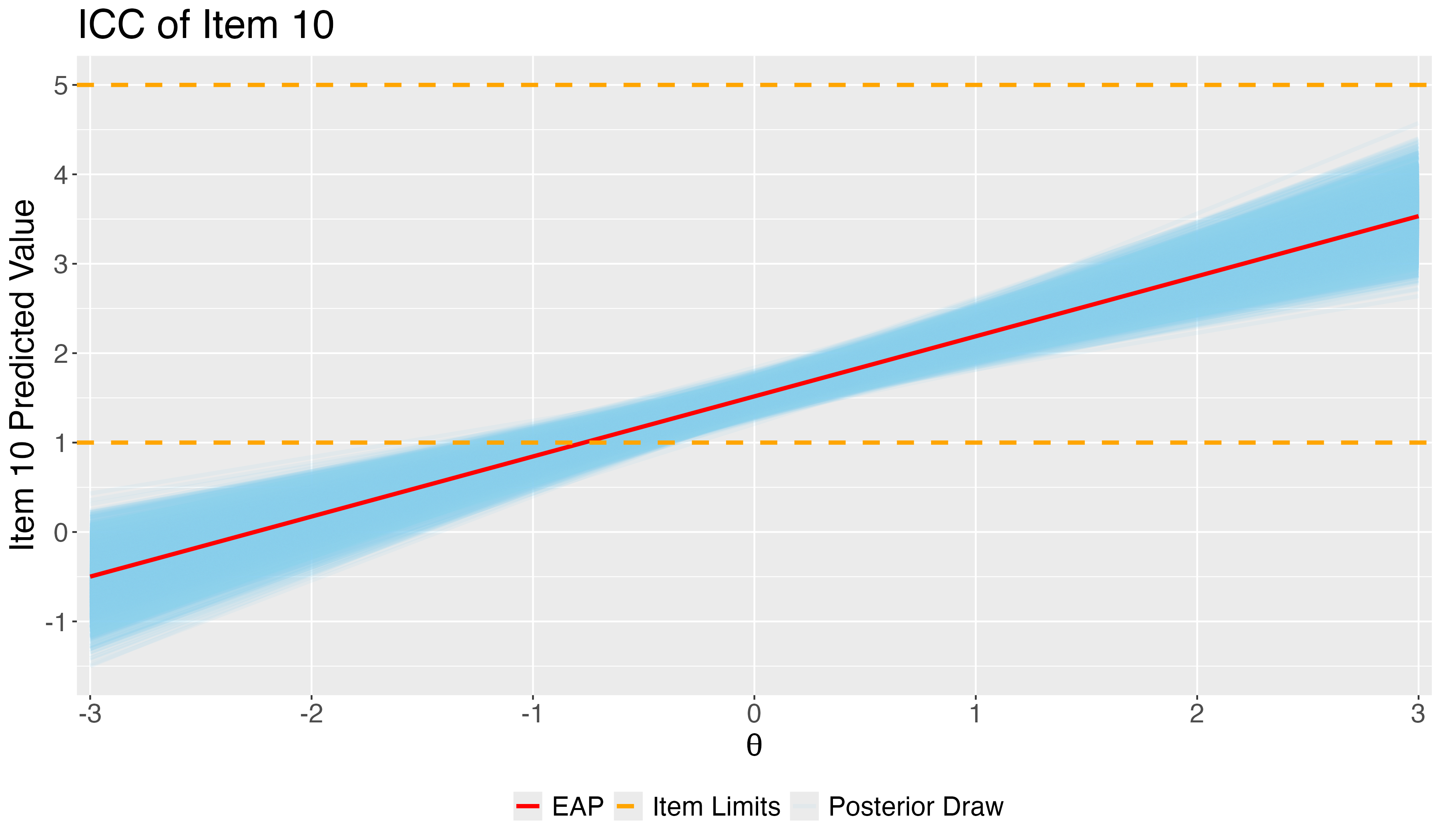
One plot that can help provide information about the item parameters is the item characteristic curve (ICC)

• Not called this in Confirmatory Factor Analysis (but equivalent)

• The ICC is the plot of the expected value of the response conditional on the value of the latent traits, for a range of latent trait values

  E(Ypi∣θp)=μi+λiθp

  ICC=f(E(Ypi∣θp),θp)

• Because we have sampled values for each parameter, we can plot one ICC for each posterior draw

Posterior ICC Plots: Difficulty and Discrimination of Item 10

• Using ICC, we can check the predicted response on item 10 given one’s belief in conspiracy.

Review Our R files

Next Class

• More results from conspiracy data

• Compare results to blavaan package