Lecture 09

Generalized Measurement Models: Modeling Observed Dichotomous Data

Jihong Zhang

Educational Statistics and Research Methods

Previous Class

1. Dive deep into factor scoring
2. Show how different initial values affect Bayesian model estimation
3. Show how parameterization differs for standardized latent variables vs. marker item scale identification

Today’s Lecture Objectives

1. Show how to estimate unidimensional latent variable models with dichotomous data
   1. Also know as Item response theory (IRT) or Item factor analysis (IFA)
2. Show how to estimate different parameterizations of IRT/IFA models
3. Describe how to obtain IRT/IFA auxiliary statistics from Markov Chains
4. Show variations of various dichotomous-data models.

Example Data: Conspiracy Theories

• Today’s example is from a bootstrap resample of 177 undergraduate students at a large state university in the Midwest.
• The survey was a measure of 10 questions about their beliefs in various conspiracy theories that were being passed around the internet in the early 2010s
• All item responses were on a 5-point Likert scale with:
  1. Strong Disagree → 0
  2. Disagree → 0
  3. Neither Agree nor Disagree → 0
  4. Agree → 1
  5. Strongly Agree → 1
• The purpose of this survey was to study individual beliefs regarding conspiracies.
• Our purpose in using this instrument is to provide a context that we all may find relevant as many of these conspiracies are still prevalent.

Make Our Data Dichotomous (not a good idea in practice)

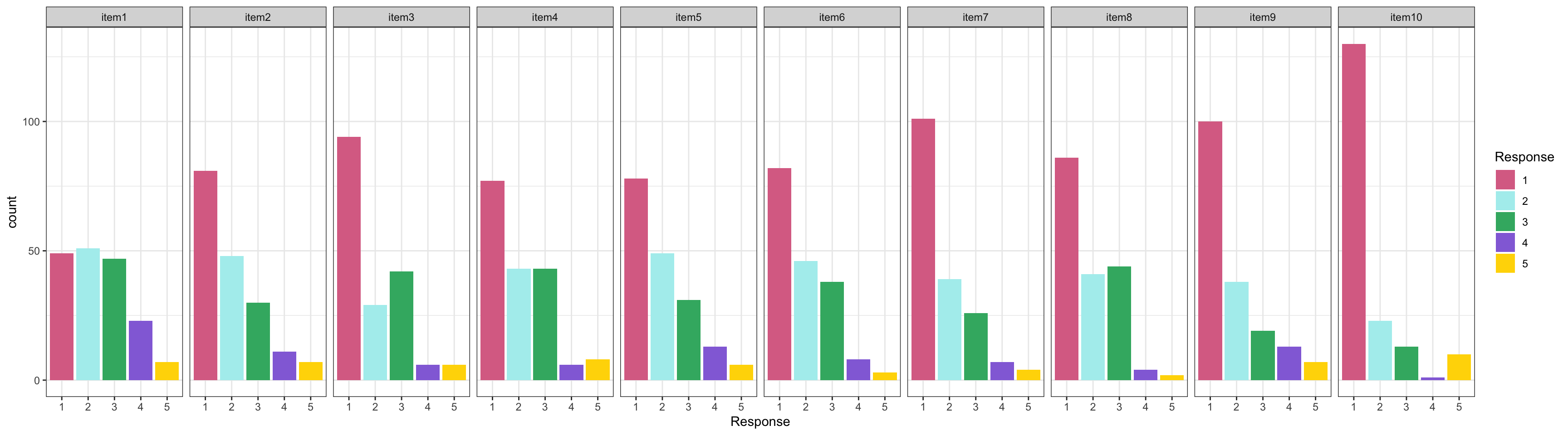
To show dichotomous-data models with our data, we will arbitrarilly dichotomize our item responses:

• {0}: Response is Strongly disagree or disagree, or Neither (1-3)

• {1}: Response is Agree, or Strongly agree (4-5)

Now, we could argue that a 1 represents someone who agrees with a statement and 0 represents someone who disagrees or is neutral.

Note that this is only for illustrative purpose, such dichotomization shouldn’t be done because

• There are distributions for multinomial categories

• The results will reflect more of our choice for 0/1

But we first learn dichotomous data models before we get to models for polytomous models.

Examining Dichotomous Data

── Attaching core tidyverse packages ──────────────────────── tidyverse 2.0.0 ──
✔ dplyr     1.1.4     ✔ readr     2.1.5
✔ forcats   1.0.0     ✔ stringr   1.5.1
✔ ggplot2   3.5.1     ✔ tibble    3.2.1
✔ lubridate 1.9.4     ✔ tidyr     1.3.1
✔ purrr     1.0.4     
── Conflicts ────────────────────────────────────────── tidyverse_conflicts() ──
✖ dplyr::filter() masks stats::filter()
✖ dplyr::lag()    masks stats::lag()
ℹ Use the conflicted package (<http://conflicted.r-lib.org/>) to force all conflicts to become errors

Attaching package: 'kableExtra'


The following object is masked from 'package:dplyr':

    group_rows


here() starts at /Users/jihong/Documents/Projects/website-jihong

Loading required package: Rcpp

This is blavaan 0.5-8

On multicore systems, we suggest use of future::plan("multicore") or
  future::plan("multisession") for faster post-MCMC computations.

Note

These items have a relatively low proportion of people agreeing with each conspiracy statement

• Highest mean: .69

• Lowest mean: .034

Dichotomous Data Distribution: Bernoulli

The Bernoulli distribution is a one-trial version of the Binomial distribution

• Sample space (support) Y∈0,1

The probability mass function:

P(Y=y)=πy(1−π)1−y

The Bernoulli distribution has only one parameter: π (typically, known as the probability of success: Y=1)

• Mean of the distribution: E(Y)=π

• Variance of the distribution: Var(Y)=π(1−π)

Definition: Dichotomous vs. Binary

Note the definitions of some of the words for data with two values:

• Dichotomous: Taking two values (without numbers attached)

• Binary: either zero or one

Therefore:

1. Not all dichotomous variable are binary, i.e., {2,7} is a dichotomous but not binary variable
2. All binary variables are dichotomous

Finally:

1. Bernoulli distributions are for binary variables
2. Most dichotomous variables can be recorded as binary variables without loss of model effects

Models with Bernoulli Distributions

Generalized linear models using Bernoulli distributions put a linear model onto a transformation of the mean

• Link function maps the mean E(Y) from its original range of [0,1] to (-∞, ∞);

• For an unconditional (empty) model, this is shown here:

f(E(Y))=f(π)

Link Functions for Bernoulli Distributions

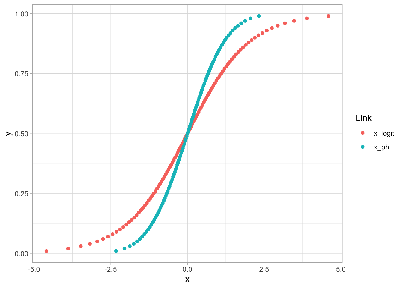
Common choices for the link function in latent variable modeling:

1. Logit (or log odds):

f(π)=log(π1−π)

2. Probit:

f(π)=Φ−1(π)

Where Φ is the inverse cumulative distribution of a standard normal distribution

Φ(Z)=∫Z−∞1√2πexp(−x22)dx

Visualization of Logit and Probit

Less Common Link Functions

In the generalized linear models literature, there are a number of different link functions:

• Log-log: f(π)=−log(−log(π))

• Complementary Log-log: f(π)=log(−log(1−π))

Most of these seldom appear in latent variable models

• Each has a slightly different curve shape

Inverse Link Functions

Our latent variable models will be defined on the scale of the link function

• Sometimes we wish to convert back to the scale of the data

• Example: Test characteristic curves mapping θp onto an expected test score

For this, we need the inverse link function

• Logit (or log odds) link function:

logit(π)=log(π1−π)

• Logit (or log odds) inverse link function:

π=exp(logit(π))1+exp(logit(π))=11+exp(−logit(π))=(1+exp(−logit(π)))−1

Latent Variable Models with Bernoulli Distributions

Define Latent Variable Models with Bernoulli Distributions

To define a LVM for binary responses using a Bernoulli Distribution

• To start, we will use the logit link function

• We will begin with the linear predictor we had from the normal distribution models (Confirmatory factor analysis: μi+λiθp)

For an item i and a person p, the model becomes:

P(Ypi=1|θp)=logit−1(μi+λiθp)

• Note: the mean πi is replaced by P(Ypi=1|θp)

  • This is the mean of the observed variable, conditional on θp;

• The item intercept (easiness, location) is μi: the expected logit when θp=0

• The item discrimination is λi: the change in the logit for a one-unit increase in θp

Extension: A more general form

A 3-PL Item Response Theory Model with same statistical form but different notations:

P(Ypi=1|θp,ci,ai,bj)=ci+(1−ci)logit−1(αiθp+di)

P(Ypi=1|θp,ci,ai,bj)=ci+(1−ci)logit−1(αi(θp−bi))

where

• θp is the latent variable for examinee p, representing the examinee’s proficiency such that higher values indicate more proficency

• ai, di, ci are item parameters:

  • ai: the capability of item to discriminate between examinees with lower and higher values along the latent variables;

  • di: item “easiness”

  • bi: item “difficulty”, bi=di/(−ai)

  • ci: “pseudo-guessing” parameter – examinees with low proficiency may have a nonzero probability of a correct response due to guessing

Model Family Names

Depending on your field, the model from the previous slide can be called:

• The two-parameter logistic (2PL) model with slope/intercept parameterization

• An item factor model

These names reflect the terms given to the model in diverging literature:

• 2PL: Education measurement

Birnbaum, A. (1968). Some Latent Trait Models and Their Use in Inferring an Examinee’s Ability. In F. M. Lord & M. R. Novick (Eds.), Statistical Theories of Mental Test Scores (pp. 397-424). Reading, MA: Addison-Wesley.

• Item factor analysis: Psychology

Christofferson, A.(1975). Factor analysis of dichotomous variables. Psychometrika , 40, 5-22.

Estimation methods are the largest difference between the two families.

Differences from Normal Distributions

Recall our normal distribution models:

Ypi=μi+λiθp+ep,i;ep,i∼N(0,ψ2i)

Compared to our Bernoulli distribution models:

logit(P(Ypi=1))=μi+λiθp

Differences:

1. No residual (unique) variance components ψ2i in Bernoulli distribution;
2. Only one parameter in the distribution; variance is a function of the mean;
3. Identity link function in normal distribution: f(E(Ypi|θp))=E(Ypi|θp)
   • Model scale and data scale are the same
4. Logit link function in Bernoulli distribution
   • Model scale is different from data scale

From Model Scale to Data Scale

Commonly, the IRT or IFA model is shown on the data scale (using the inverse link function):

P(Ypi=1)=exp(μi+λiθp)1+exp(μi+λiθp)

The core of the model (the terms in the exponent on the right-hand side) is the same

Models are equivalent:

1. P(Ypi=1) is on the data scale;
2. logit(P(Ypi=1)) is on the model (link) scale;

Modeling All Data

As with the normal distribution (CFA) models, we use the Bernoulli distribution for all observed variables:

logit(P(Yp1=1))=μ1+λ1θplogit(P(Yp2=1))=μ2+λ2θplogit(P(Yp3=1))=μ3+λ3θplogit(P(Yp4=1))=μ4+λ4θplogit(P(Yp5=1))=μ5+λ5θp…logit(P(Yp10=1))=μ10+λ10θp

Measurement Model Analysis Procedure

1. Specify model
2. Specify scale identification method for latent analysis
3. Estimate model
4. Examine model-data fit
5. Iterate between steps 1-4 until adequate fit is achieved

Measurement Model Auxiliary Steps:

1. Score estimation (and secondary analysis with scores)
2. Item evaluation
3. Scale construction
4. Equating
5. Measurement invariance / differential item functioning

Model Specification

The set of equations on the previous slide formed Step #1 of the Measurement Model Analysis

1. Specify Model

The next step is:

2. Specify scale identification method for latent variables

We will initially assume θp∼N(0,1), which allows us to estimate all item parameters of the model, that we call standardization

Likelihood Functions

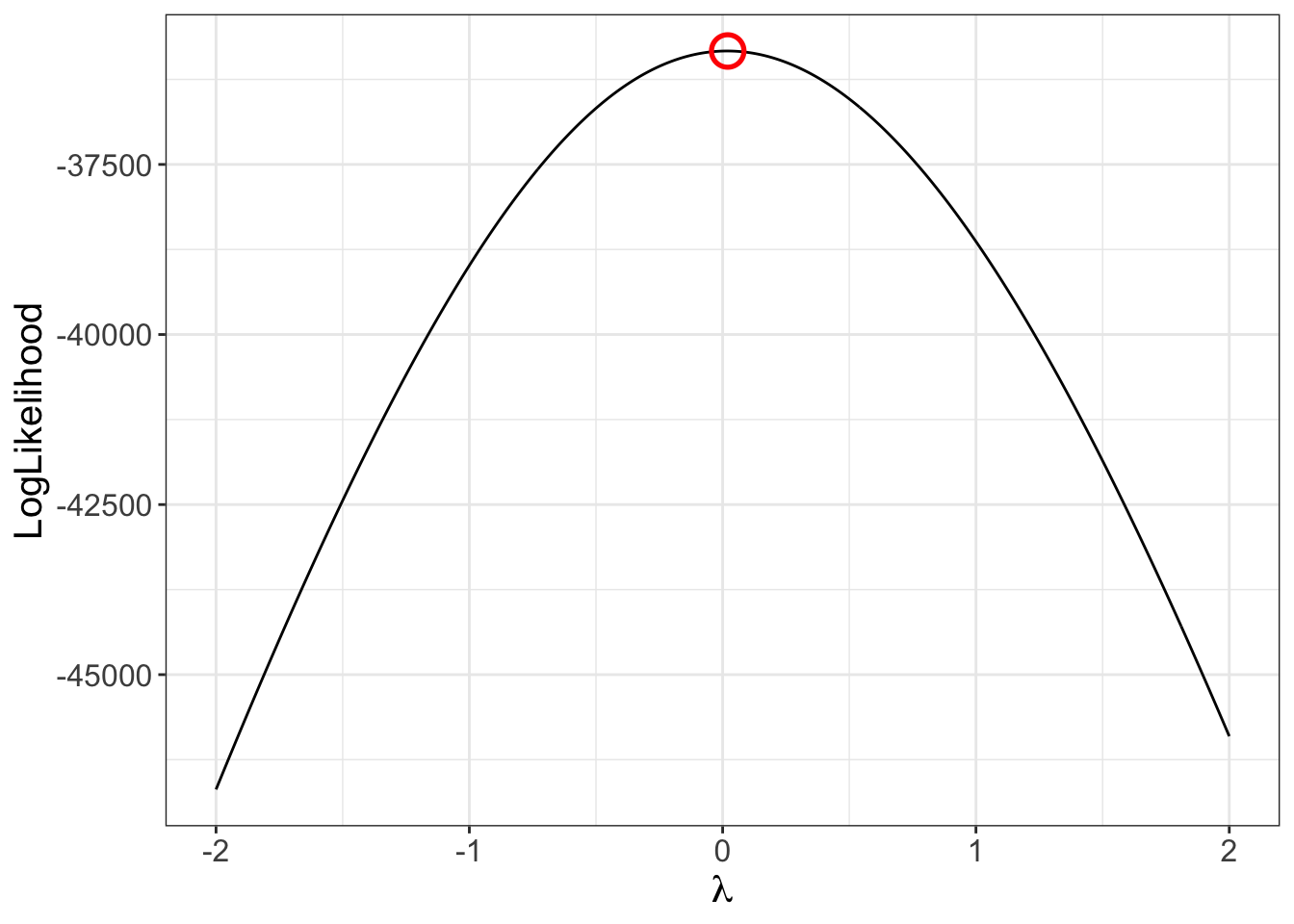
The likelihood of item 1 is the function of production of all individuals’ responses:

f(Ypi|λ1)=P∏p=1(πp1)Yp1(1−πp1)1−Yp1(1)

To simplify Equation 1, we take the log:

logf(Ypi|λ1)=ΣPp−1log[(πp1)Ypi(1−πp1)1−Ypi](2)

Since we know from logit function that:

πpi=exp(μ1+λ1θp)1+exp(μ1+λ1θp)

Which then becomes:

logf(Ypi|λ1)=ΣPp−1log[(exp(μ1+λ1θp)1+exp(μ1+λ1θp))Ypi(1−exp(μ1+λ1θp)1+exp(μ1+λ1θp))1−Ypi]

Model (Data) Log Likelihood Functions

As an example for λ1:

Model (Data) Log Likelihood Function for θ

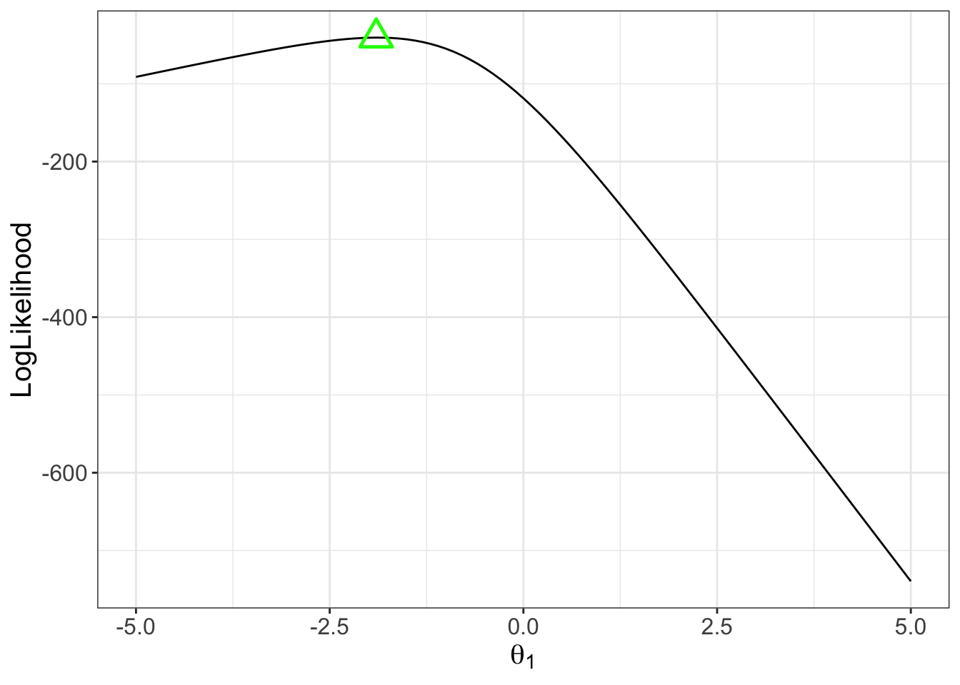
For each person, the same model likelihood function is used

• Only now it varies across each item response

• Example: Person 1

f(Y1i|θ1)=I∏i=1(π1i)Y1i(1−π1i)1−Y1i

Implementing Bernoulli Outcomes in Stan

Stan’s model Block

model {
  
  lambda ~ multi_normal(meanLambda, covLambda); // Prior for item discrimination/factor loadings
  mu ~ multi_normal(meanMu, covMu);             // Prior for item intercepts
  
  theta ~ normal(0, 1);                         // Prior for latent variable (with mean/sd specified)
  
  for (item in 1:nItems){
    Y[item] ~ bernoulli_logit(mu[item] + lambda[item]*theta);
  }
  
}

For logit models without lower / upper asymptote parameters, Stan has a convenient bernoulli_logit function

• Automatically has the link function embedded

• The catch: The data has to be defined as an integer

Also, note that there are few differences from the model with normal outcomes (CFA)

• No ψ parameters

Stan’s parameters Block

parameters {
  vector[nObs] theta;                // the latent variables (one for each person)
  vector[nItems] mu;                 // the item intercepts (one for each item)
  vector[nItems] lambda;             // the factor loadings/item discriminations (one for each item)
}

Only change from normal outcomes (CFA) model:

• No ψ (psi) parameters

Stan’s data{} Block

data {
  int<lower=0> nObs;                            // number of observations
  int<lower=0> nItems;                          // number of items
  array[nItems, nObs] int<lower=0, upper=1>  Y; // item responses in an array

  vector[nItems] meanMu;             // prior mean vector for intercept parameters
  matrix[nItems, nItems] covMu;      // prior covariance matrix for intercept parameters
  
  vector[nItems] meanLambda;         // prior mean vector for discrimination parameters
  matrix[nItems, nItems] covLambda;  // prior covariance matrix for discrimination parameters
}

One difference from normal outcome model:

array[nItems, nObs] int<lower=0, upper=1> Y;

• Arrays are types of matrices (with more than two dimensions possible)

  • Allows for different types of data (here Y are integers)

    • Integer-valued variables needed for bernoulli_logit() function

• Arrays are row-major (meaning order of items and persons is switched)

  • Can define differently

Change to Data List for Stan Import

The switch of items and observations in the array statement means the data imported have to be transposed:

modelIRT_2PL_SI_data = list(
  nObs = nObs,
  nItems = nItems,
  Y = t(conspiracyItemsDichtomous), 
  meanMu = muMeanVecHP,
  covMu = muCovarianceMatrixHP,
  meanLambda = lambdaMeanVecHP,
  covLambda = lambdaCovarianceMatrixHP
)

Running the Model in Stan

The Stan program takes longer to run than in linear models:

• Number of parameters: 197

  • 10 observed variables: μi and λi for i=1…10

  • 177 latent variables: θp for p=1…177

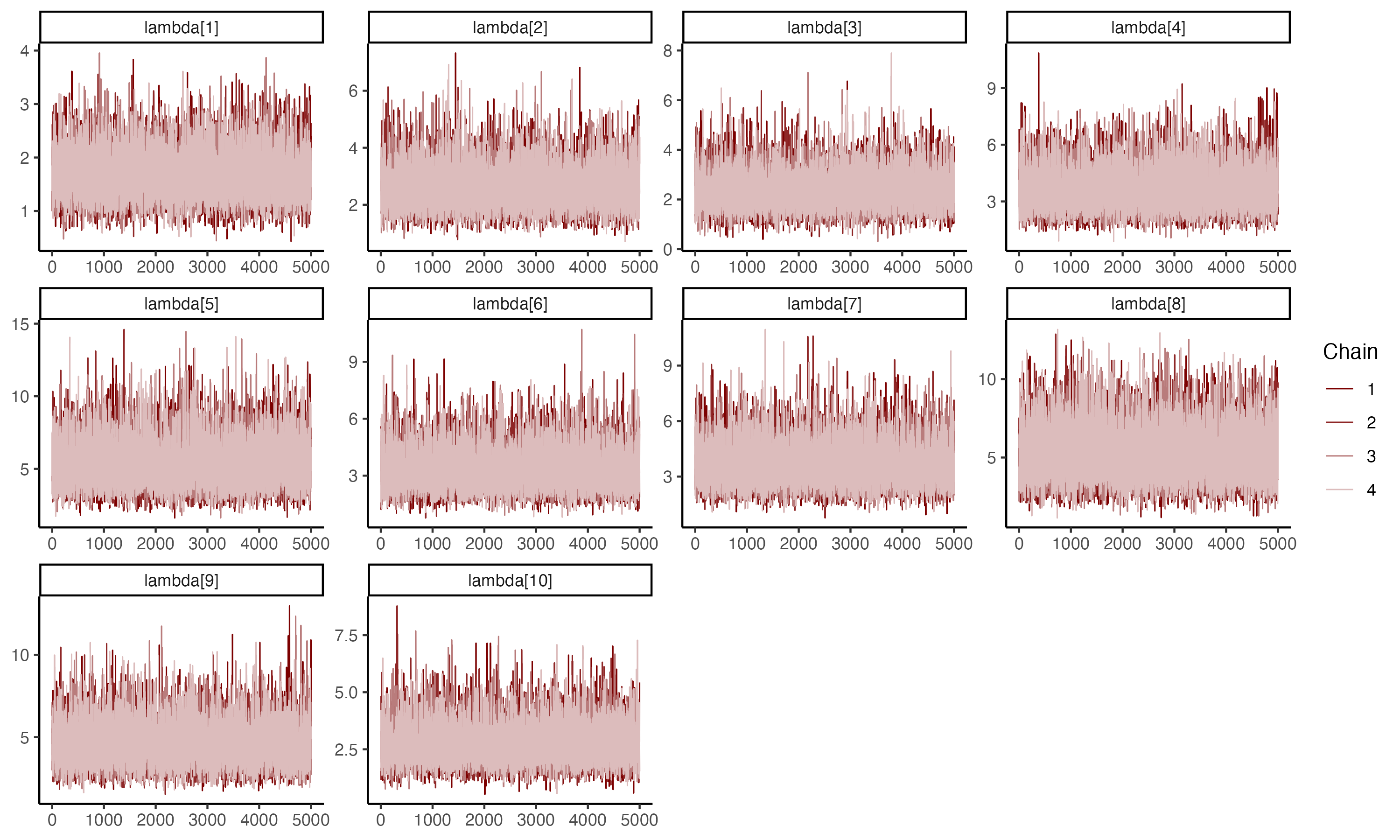
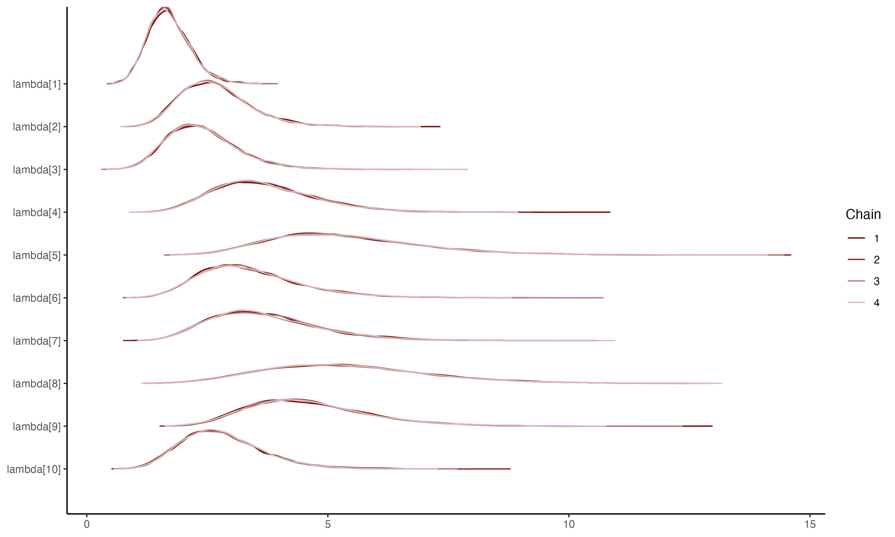
• cmdstanr samples call:

```{r}
#| eval: false
modelIRT_2PL_SI_samples = modelIRT_2PL_SI_stan$sample(
  data = modelIRT_2PL_SI_data,
  seed = 02112022,
  chains = 4,
  parallel_chains = 4,
  iter_warmup = 5000,
  iter_sampling = 5000,
  init = function() list(lambda=rnorm(nItems, mean=5, sd=1))
)
```

• Note: typically, longer chains are needed for larger models like this

• Note: Starting values added (mean of 5 is due to logit function limits)

  • Helps keep definition of parameters (stay away from opposite mode)

  • Too large of value can lead to NaN values (exceeding numerical precision)

Model Results

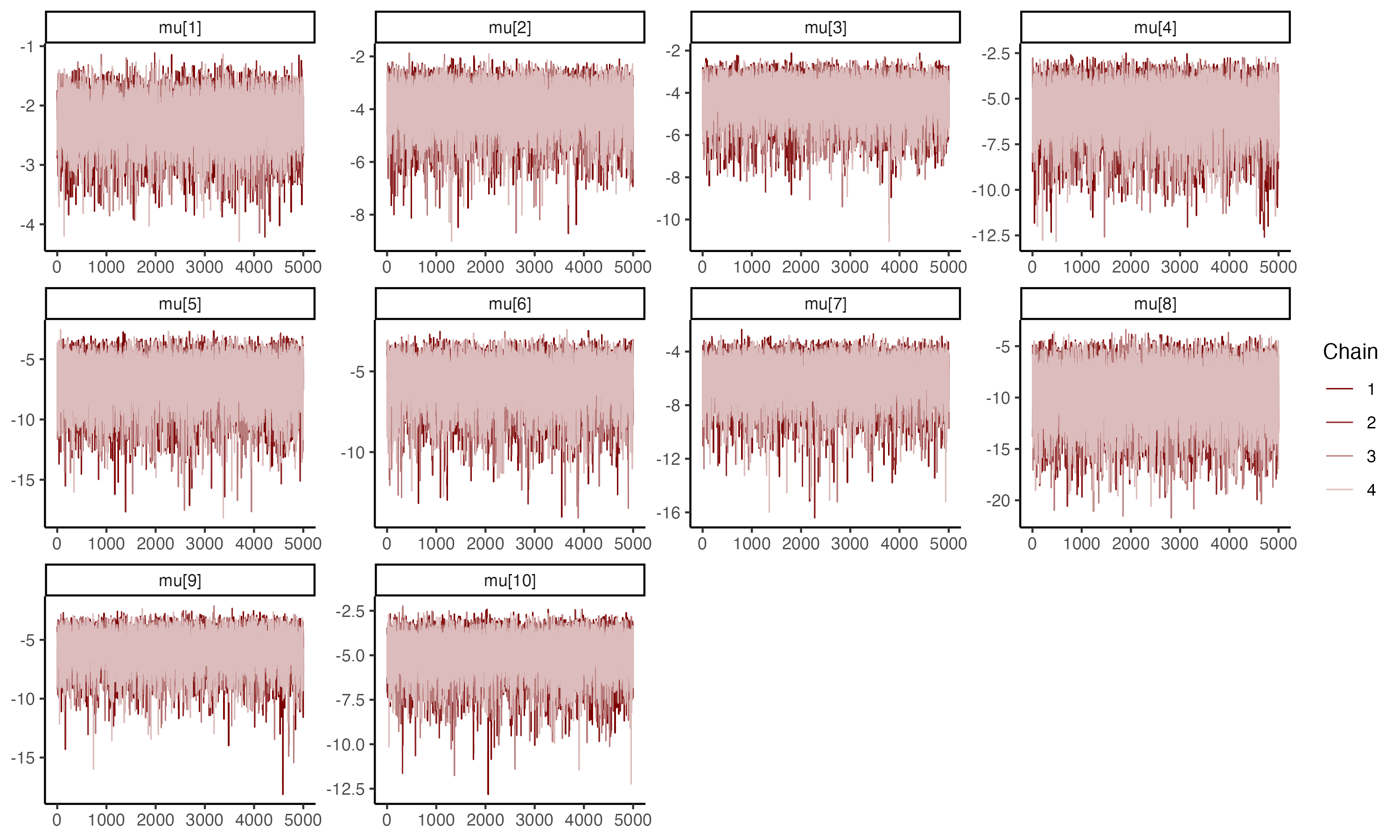
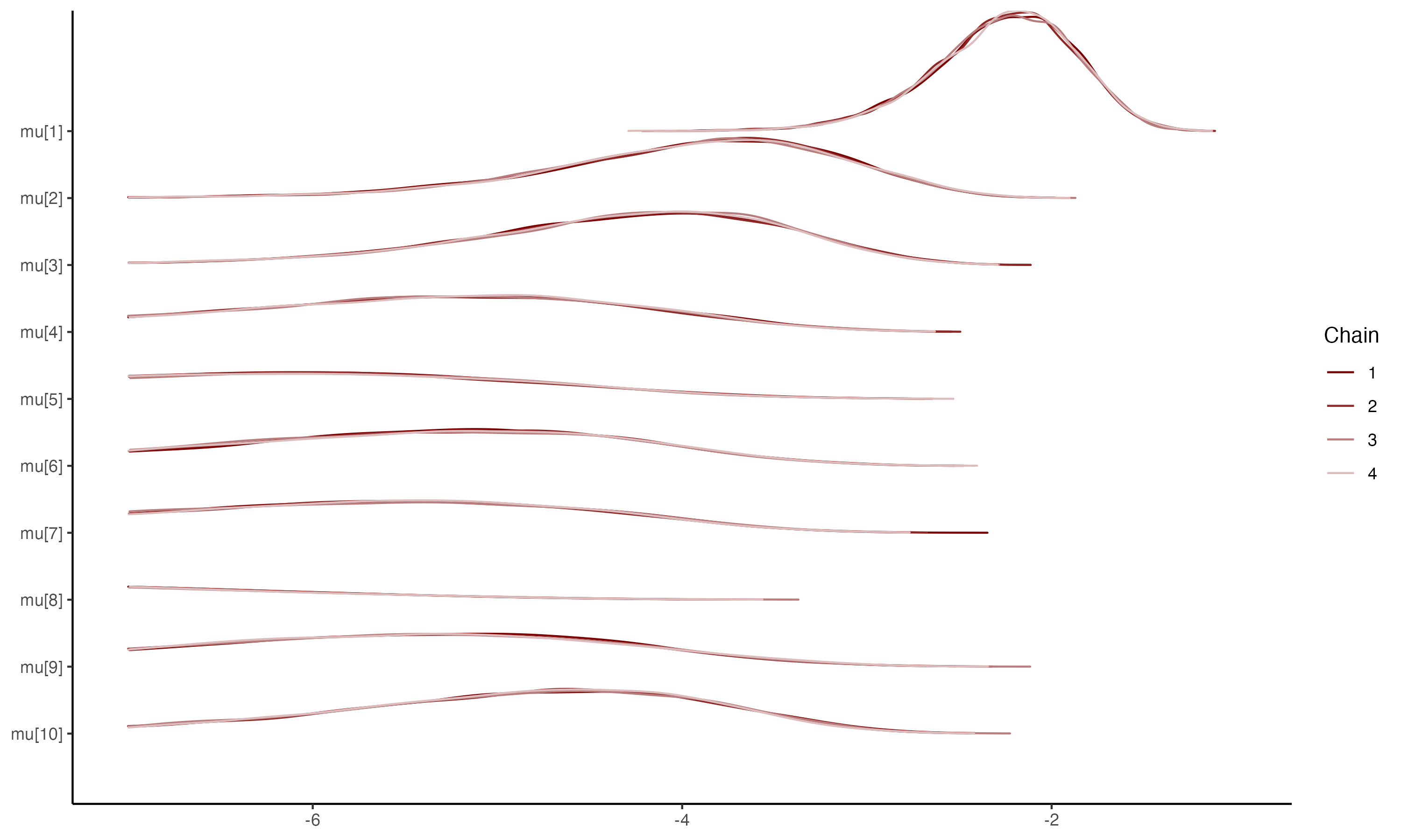
Warning: package 'cmdstanr' was built under R version 4.4.3

This is cmdstanr version 0.8.1

- CmdStanR documentation and vignettes: mc-stan.org/cmdstanr

- CmdStan path: /Users/jihong/.cmdstan/cmdstan-2.36.0

- CmdStan version: 2.36.0

Check convergence with ˆR (PSRF):

      rhat       
 Min.   :0.9999  
 1st Qu.:1.0001  
 Median :1.0002  
 Mean   :1.0002  
 3rd Qu.:1.0004  
 Max.   :1.0010  

• Item Parameter Results:

# A tibble: 20 × 10
   variable    mean median    sd   mad     q5   q95  rhat ess_bulk ess_tail
   <chr>      <dbl>  <dbl> <dbl> <dbl>  <dbl> <dbl> <dbl>    <dbl>    <dbl>
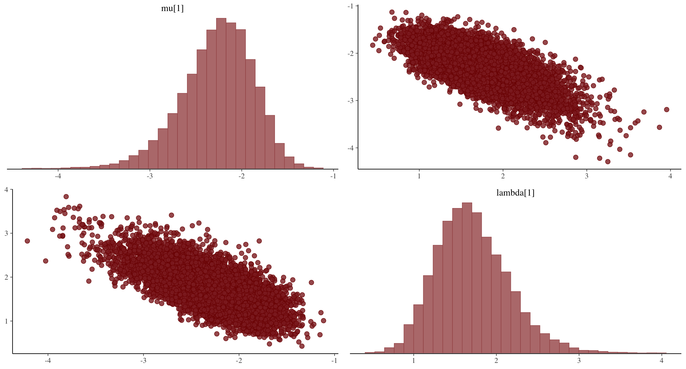
 1 mu[1]      -2.27  -2.23 0.389 0.373  -2.96 -1.69  1.00   10459.   10267.
 2 mu[2]      -3.98  -3.87 0.825 0.767  -5.47 -2.82  1.00   10367.    9220.
 3 mu[3]      -4.36  -4.24 0.909 0.853  -6.03 -3.11  1.00    9487.    8934.
 4 mu[4]      -5.62  -5.44 1.34  1.26   -8.07 -3.77  1.00   11126.    9699.
 5 mu[5]      -6.91  -6.62 1.90  1.77  -10.4  -4.36  1.00    9307.    9026.
 6 mu[6]      -5.70  -5.48 1.41  1.29   -8.30 -3.83  1.00    9499.    8609.
 7 mu[7]      -6.10  -5.86 1.56  1.44   -8.99 -4.01  1.00    9993.    8759.
 8 mu[8]      -9.71  -9.42 2.62  2.60  -14.5  -5.92  1.00   14173.   11574.
 9 mu[9]      -5.87  -5.66 1.49  1.38   -8.65 -3.82  1.00   10408.    9160.
10 mu[10]     -4.99  -4.83 1.12  1.04   -7.01 -3.46  1.00   10083.    8465.
11 lambda[1]   1.71   1.67 0.435 0.423   1.06  2.47  1.00    7367.    9356.
12 lambda[2]   2.67   2.59 0.740 0.692   1.64  4.02  1.00    7839.    8497.
13 lambda[3]   2.42   2.33 0.759 0.705   1.36  3.80  1.00    7624.    7123.
14 lambda[4]   3.71   3.57 1.08  1.03    2.20  5.68  1.00    8935.    9175.
15 lambda[5]   5.43   5.19 1.62  1.51    3.23  8.41  1.00    8350.    9162.
16 lambda[6]   3.40   3.24 1.08  0.993   1.94  5.40  1.00    7379.    7790.
17 lambda[7]   3.71   3.55 1.16  1.09    2.11  5.84  1.00    8614.    8116.
18 lambda[8]   5.41   5.24 1.70  1.67    2.93  8.51  1.00   11540.   11101.
19 lambda[9]   4.64   4.47 1.29  1.21    2.86  7.00  1.00    8560.    9090.
20 lambda[10]  2.83   2.72 0.874 0.825   1.59  4.41  1.00    8457.    8456.

Modeling Strategy vs. Didactic Strategy

At this point, one should investigate model fit of the model we just ran (PPP, WAIC, LOO)

• If the model does not fit, then all model parameters could be biased

  • Both item parameters and person parameters (μi, λi, θp)

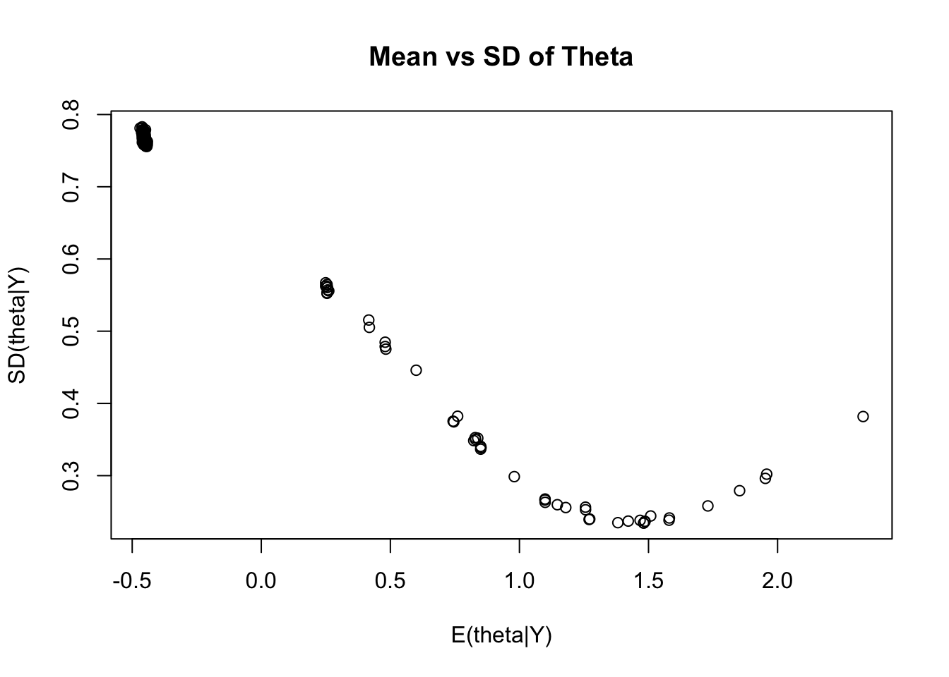
• Moreover, the uncertainty accompanying each parameter (the posterior standard deviation) may also be biased

  • Especially bad for psychometric models as we quantify reliability with these numbers

Investigating Item Parameters

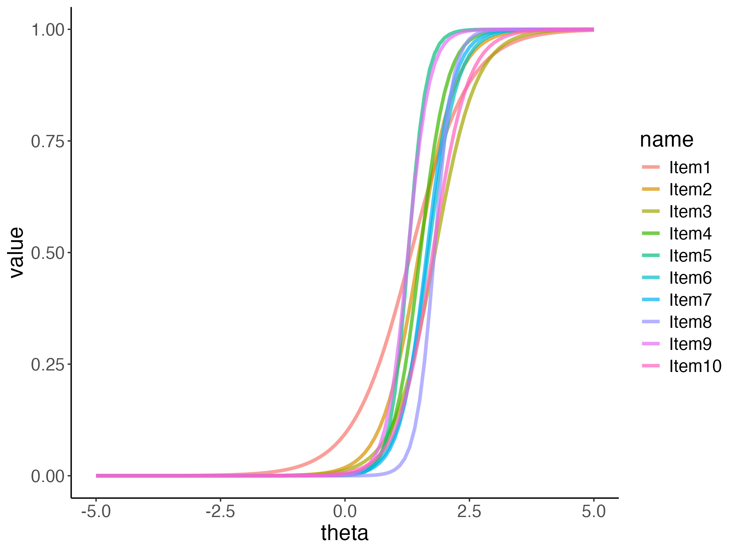
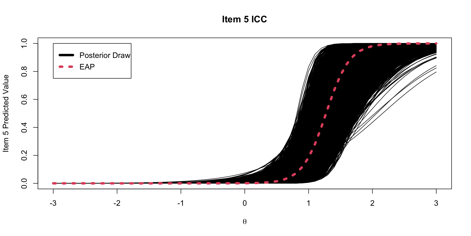
One plot that can help provide information about the item parameters is the item characteristic curve (ICC)

• The ICC is the plot of the expected value of the response conditional on the value of the latent traits, for a range of latent trait values

E(Ypi|θp)=exp(μi+λiθp)1+exp(μi+λiθp)

• Because we have sampled values for each parameter, we can plot one ICC for each posterior draws

Posterior ICC Plots

ICC for 10 items

Item 5 ICC

Investigating the Item Parameters

Trace plots for μi

Density plots for μi

Trace plots for λi

Density plots for λi

Bivariate plots for μi and λi

Latent Variables

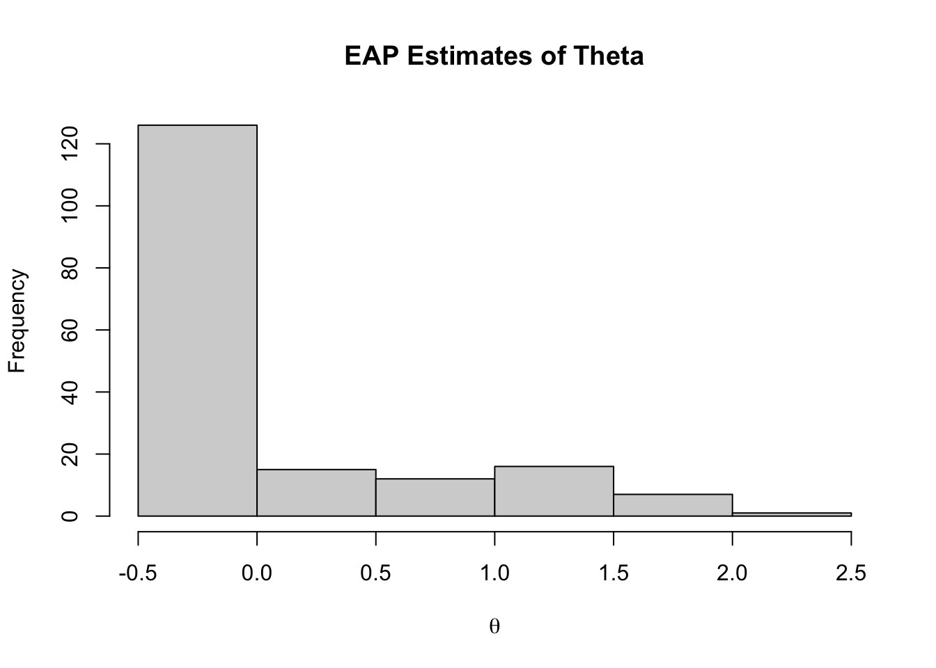
# A tibble: 177 × 10
    variable     mean median    sd   mad      q5   q95  rhat ess_bulk ess_tail
    <chr>       <dbl>  <dbl> <dbl> <dbl>   <dbl> <dbl> <dbl>    <dbl>    <dbl>
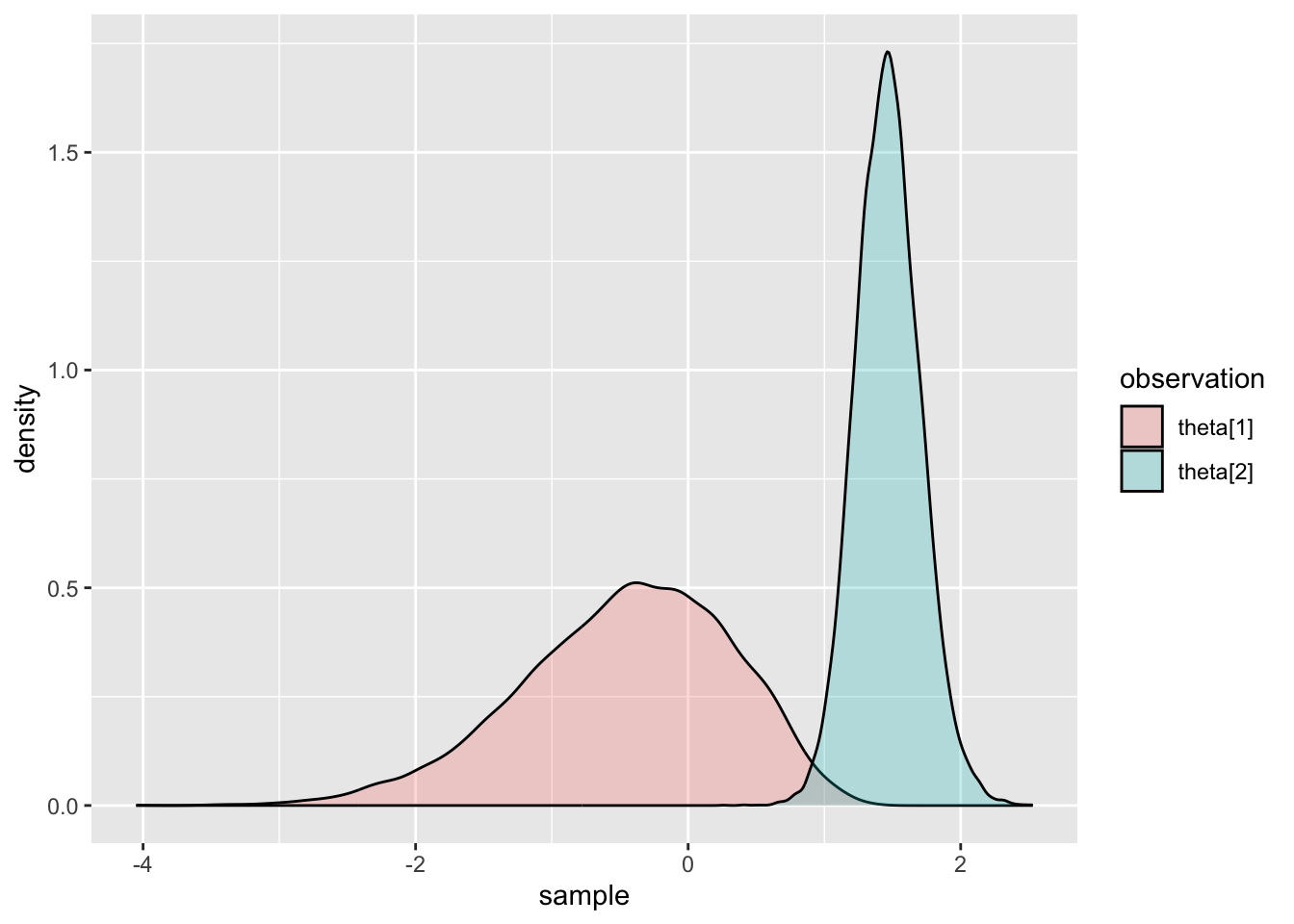
  1 theta[1]   -0.457 -0.393 0.771 0.788 -1.84   0.686  1.00   30500.   13873.
  2 theta[2]    1.47   1.46  0.238 0.233  1.09   1.86   1.00    8777.   11807.
  3 theta[3]    1.51   1.50  0.244 0.241  1.12   1.92   1.00    8370.   11997.
  4 theta[4]   -0.454 -0.382 0.768 0.771 -1.84   0.671  1.00   30720.   14251.
  5 theta[5]   -0.451 -0.384 0.768 0.774 -1.83   0.680  1.00   30700.   12840.
  6 theta[6]   -0.449 -0.381 0.766 0.772 -1.81   0.681  1.00   30823.   13118.
  7 theta[7]    0.261  0.343 0.556 0.527 -0.772  1.02   1.00   20344.   12386.
  8 theta[8]    0.480  0.554 0.485 0.434 -0.430  1.13   1.00   19416.   11766.
  9 theta[9]   -0.461 -0.396 0.761 0.785 -1.81   0.662  1.00   32046.   14796.
 10 theta[10]  -0.455 -0.391 0.774 0.802 -1.84   0.677  1.00   31176.   14674.
 11 theta[11]  -0.450 -0.385 0.762 0.787 -1.80   0.673  1.00   30931.   13838.
 12 theta[12]  -0.448 -0.379 0.767 0.786 -1.83   0.676  1.00   32110.   13432.
 13 theta[13]  -0.449 -0.369 0.779 0.794 -1.85   0.692  1.00   33002.   12115.
 14 theta[14]  -0.463 -0.395 0.775 0.787 -1.83   0.685  1.00   32905.   13840.
 15 theta[15]  -0.458 -0.396 0.770 0.784 -1.83   0.680  1.00   30779.   14384.
 16 theta[16]  -0.454 -0.387 0.763 0.776 -1.82   0.677  1.00   32739.   14097.
 17 theta[17]  -0.459 -0.383 0.771 0.786 -1.84   0.680  1.00   31754.   14551.
 18 theta[18]  -0.455 -0.390 0.758 0.774 -1.80   0.669  1.00   30244.   12924.
 19 theta[19]   1.26   1.26  0.256 0.248  0.831  1.67   1.00    9820.   12100.
 20 theta[20]  -0.459 -0.395 0.763 0.771 -1.82   0.676  1.00   29995.   13659.
 21 theta[21]  -0.459 -0.385 0.775 0.788 -1.86   0.684  1.00   30952.   13566.
 22 theta[22]  -0.457 -0.388 0.771 0.781 -1.84   0.679  1.00   29283.   14053.
 23 theta[23]  -0.455 -0.385 0.765 0.779 -1.82   0.674  1.00   29673.   13955.
 24 theta[24]  -0.457 -0.394 0.770 0.778 -1.84   0.683  1.00   28874.   13416.
 25 theta[25]   0.250  0.328 0.562 0.533 -0.797  1.02   1.00   21958.   11757.
 26 theta[26]   1.10   1.11  0.268 0.250  0.643  1.51   1.00   13632.   12826.
 27 theta[27]   0.746  0.790 0.374 0.340  0.0633 1.27   1.00   18359.   11203.
 28 theta[28]  -0.453 -0.376 0.777 0.773 -1.87   0.688  1.00   31732.   14297.
 29 theta[29]   0.850  0.888 0.340 0.309  0.244  1.34   1.00   16689.   11256.
 30 theta[30]   1.42   1.42  0.237 0.231  1.04   1.81   1.00    8920.   11391.
 31 theta[31]  -0.457 -0.387 0.761 0.770 -1.82   0.674  1.00   32384.   15059.
 32 theta[32]  -0.458 -0.391 0.778 0.796 -1.84   0.692  1.00   33305.   12106.
 33 theta[33]  -0.456 -0.385 0.765 0.772 -1.82   0.681  1.00   30544.   14436.
 34 theta[34]  -0.454 -0.384 0.771 0.790 -1.82   0.689  1.00   30237.   14405.
 35 theta[35]  -0.457 -0.388 0.775 0.784 -1.85   0.679  1.00   31052.   15148.
 36 theta[36]  -0.457 -0.395 0.769 0.790 -1.84   0.681  1.00   32515.   13230.
 37 theta[37]  -0.451 -0.378 0.773 0.791 -1.83   0.687  1.00   32388.   14023.
 38 theta[38]  -0.461 -0.390 0.771 0.782 -1.83   0.681  1.00   30644.   13735.
 39 theta[39]  -0.455 -0.386 0.770 0.785 -1.82   0.676  1.00   28524.   13479.
 40 theta[40]  -0.459 -0.390 0.774 0.783 -1.84   0.674  1.00   30985.   14185.
 41 theta[41]  -0.455 -0.387 0.773 0.771 -1.86   0.681  1.00   32230.   13360.
 42 theta[42]  -0.461 -0.389 0.766 0.784 -1.84   0.666  1.00   29580.   13829.
 43 theta[43]  -0.450 -0.383 0.759 0.773 -1.82   0.667  1.00   31264.   14672.
 44 theta[44]  -0.450 -0.383 0.761 0.770 -1.81   0.665  1.00   31665.   13545.
 45 theta[45]   0.980  1.00  0.299 0.278  0.455  1.42   1.00   13989.   11341.
 46 theta[46]  -0.453 -0.390 0.769 0.780 -1.83   0.685  1.00   28889.   12706.
 47 theta[47]  -0.448 -0.384 0.764 0.787 -1.80   0.683  1.00   32802.   13739.
 48 theta[48]  -0.441 -0.377 0.763 0.794 -1.79   0.692  1.00   29030.   13880.
 49 theta[49]  -0.454 -0.381 0.771 0.772 -1.85   0.670  1.00   29003.   14052.
 50 theta[50]   0.851  0.886 0.339 0.307  0.241  1.34   1.00   15680.   10429.
 51 theta[51]  -0.451 -0.384 0.770 0.785 -1.83   0.684  1.00   32348.   14439.
 52 theta[52]  -0.453 -0.385 0.767 0.780 -1.82   0.675  1.00   32585.   13420.
 53 theta[53]  -0.452 -0.386 0.767 0.783 -1.81   0.680  1.00   30511.   13102.
 54 theta[54]  -0.452 -0.394 0.772 0.797 -1.82   0.701  1.00   32147.   14392.
 55 theta[55]  -0.442 -0.371 0.759 0.759 -1.79   0.676  1.00   31541.   13599.
 56 theta[56]  -0.455 -0.389 0.774 0.790 -1.83   0.689  1.00   31674.   13981.
 57 theta[57]  -0.446 -0.378 0.760 0.771 -1.80   0.666  1.00   30740.   14430.
 58 theta[58]  -0.463 -0.399 0.775 0.782 -1.84   0.681  1.00   32070.   14093.
 59 theta[59]   0.249  0.330 0.567 0.539 -0.793  1.03   1.00   21373.   11756.
 60 theta[60]  -0.451 -0.384 0.760 0.766 -1.82   0.666  1.00   29591.   12609.
 61 theta[61]   1.18   1.19  0.256 0.240  0.744  1.58   1.00   11702.   11992.
 62 theta[62]  -0.452 -0.384 0.770 0.774 -1.83   0.682  1.00   30832.   13753.
 63 theta[63]  -0.460 -0.389 0.775 0.789 -1.84   0.679  1.00   28320.   13207.
 64 theta[64]   1.10   1.11  0.263 0.249  0.650  1.51   1.00   13077.   12994.
 65 theta[65]  -0.460 -0.393 0.770 0.791 -1.83   0.684  1.00   33409.   14098.
 66 theta[66]  -0.457 -0.382 0.764 0.776 -1.84   0.665  1.00   30183.   14007.
 67 theta[67]  -0.456 -0.384 0.759 0.770 -1.82   0.670  1.00   30756.   14791.
 68 theta[68]  -0.450 -0.375 0.771 0.780 -1.84   0.684  1.00   31975.   14152.
 69 theta[69]  -0.455 -0.385 0.768 0.770 -1.83   0.678  1.00   32341.   14187.
 70 theta[70]  -0.454 -0.385 0.769 0.781 -1.83   0.674  1.00   29753.   14084.
 71 theta[71]  -0.456 -0.386 0.766 0.779 -1.82   0.673  1.00   30752.   14284.
 72 theta[72]   1.27   1.27  0.239 0.230  0.873  1.66   1.00   10442.   11963.
 73 theta[73]  -0.446 -0.380 0.764 0.770 -1.82   0.674  1.00   29411.   13401.
 74 theta[74]  -0.452 -0.388 0.766 0.777 -1.82   0.689  1.00   31288.   13629.
 75 theta[75]  -0.449 -0.381 0.760 0.768 -1.81   0.672  1.00   29867.   13113.
 76 theta[76]   2.33   2.29  0.382 0.364  1.77   3.01   1.00   10971.   12287.
 77 theta[77]  -0.469 -0.402 0.781 0.796 -1.86   0.689  1.00   26618.   13635.
 78 theta[78]   0.743  0.787 0.375 0.339  0.0574 1.27   1.00   18948.   11638.
 79 theta[79]   1.26   1.26  0.253 0.246  0.837  1.67   1.00   10294.   12686.
 80 theta[80]  -0.452 -0.384 0.767 0.779 -1.83   0.673  1.00   32540.   14006.
 81 theta[81]  -0.459 -0.393 0.767 0.784 -1.83   0.672  1.00   31333.   13892.
 82 theta[82]  -0.454 -0.389 0.762 0.778 -1.81   0.675  1.00   34913.   14416.
 83 theta[83]  -0.455 -0.383 0.771 0.788 -1.83   0.685  1.00   30564.   14183.
 84 theta[84]   1.58   1.57  0.241 0.238  1.20   1.99   1.00    8749.   10292.
 85 theta[85]   0.482  0.551 0.475 0.440 -0.401  1.13   1.00   19151.   12502.
 86 theta[86]  -0.455 -0.390 0.765 0.784 -1.81   0.686  1.00   32271.   13338.
 87 theta[87]   0.419  0.493 0.505 0.474 -0.520  1.10   1.00   18565.   12167.
 88 theta[88]  -0.447 -0.370 0.761 0.761 -1.80   0.684  1.00   31629.   14820.
 89 theta[89]  -0.457 -0.390 0.772 0.779 -1.83   0.676  1.00   30883.   12640.
 90 theta[90]   0.250  0.331 0.563 0.537 -0.787  1.03   1.00   23189.   12188.
 91 theta[91]  -0.450 -0.382 0.768 0.786 -1.82   0.682  1.00   32606.   14400.
 92 theta[92]   1.15   1.16  0.260 0.250  0.708  1.55   1.00   11996.   11953.
 93 theta[93]  -0.457 -0.384 0.772 0.779 -1.84   0.689  1.00   32992.   14280.
 94 theta[94]   1.95   1.93  0.296 0.287  1.51   2.47   1.00    8267.   11311.
 95 theta[95]   1.48   1.48  0.235 0.227  1.11   1.88   1.00    8689.   11447.
 96 theta[96]  -0.456 -0.386 0.774 0.778 -1.83   0.682  1.00   28902.   14284.
 97 theta[97]  -0.463 -0.390 0.779 0.788 -1.85   0.686  1.00   32083.   14443.
 98 theta[98]  -0.457 -0.380 0.775 0.784 -1.85   0.675  1.00   31768.   15188.
 99 theta[99]  -0.458 -0.386 0.772 0.771 -1.85   0.672  1.00   31462.   13287.
100 theta[100] -0.458 -0.392 0.775 0.791 -1.84   0.689  1.00   33029.   14353.
101 theta[101] -0.456 -0.388 0.769 0.794 -1.82   0.689  1.00   31082.   14923.
102 theta[102]  1.85   1.84  0.279 0.274  1.42   2.33   1.00    7859.   11726.
103 theta[103] -0.451 -0.384 0.764 0.786 -1.81   0.675  1.00   32884.   15056.
104 theta[104]  1.49   1.48  0.236 0.230  1.11   1.88   1.00    9078.   11160.
105 theta[105] -0.456 -0.392 0.771 0.791 -1.84   0.673  1.00   32176.   15433.
106 theta[106]  0.830  0.868 0.350 0.321  0.201  1.33   1.00   15239.   11297.
107 theta[107]  1.58   1.57  0.238 0.234  1.20   1.99   1.00    8139.   10489.
108 theta[108]  0.255  0.335 0.561 0.536 -0.779  1.03   1.00   23309.   11922.
109 theta[109] -0.455 -0.380 0.770 0.779 -1.85   0.680  1.00   29033.   13002.
110 theta[110] -0.459 -0.389 0.776 0.780 -1.86   0.684  1.00   31004.   12993.
111 theta[111] -0.456 -0.388 0.762 0.774 -1.81   0.676  1.00   30938.   15131.
112 theta[112]  0.255  0.329 0.553 0.536 -0.763  1.02   1.00   23485.   13098.
113 theta[113] -0.452 -0.383 0.767 0.783 -1.82   0.691  1.00   32840.   14285.
114 theta[114] -0.451 -0.383 0.764 0.773 -1.80   0.678  1.00   29074.   13827.
115 theta[115]  1.49   1.48  0.237 0.231  1.11   1.88   1.00    8501.   11957.
116 theta[116] -0.451 -0.379 0.776 0.794 -1.85   0.681  1.00   32045.   14303.
117 theta[117] -0.457 -0.388 0.767 0.777 -1.82   0.680  1.00   29228.   14169.
118 theta[118] -0.454 -0.388 0.769 0.786 -1.82   0.690  1.00   32596.   14241.
119 theta[119] -0.458 -0.394 0.772 0.794 -1.83   0.680  1.00   31877.   14171.
120 theta[120] -0.452 -0.392 0.761 0.785 -1.81   0.675  1.00   29645.   13521.
121 theta[121]  0.600  0.665 0.446 0.407 -0.230  1.21   1.00   17302.   11767.
122 theta[122]  0.255  0.333 0.565 0.532 -0.792  1.03   1.00   21975.   11096.
123 theta[123] -0.448 -0.384 0.757 0.771 -1.79   0.666  1.00   32792.   13790.
124 theta[124] -0.453 -0.380 0.771 0.789 -1.83   0.676  1.00   30435.   14634.
125 theta[125] -0.455 -0.384 0.766 0.785 -1.82   0.670  1.00   29946.   12441.
126 theta[126]  0.256  0.336 0.561 0.528 -0.778  1.03   1.00   23100.   11474.
127 theta[127]  0.829  0.867 0.353 0.324  0.199  1.33   1.00   15269.   11395.
128 theta[128] -0.461 -0.392 0.768 0.779 -1.84   0.684  1.00   29751.   14796.
129 theta[129] -0.452 -0.386 0.762 0.766 -1.81   0.679  1.00   28945.   13926.
130 theta[130]  1.73   1.72  0.258 0.250  1.33   2.18   1.00    7808.   11121.
131 theta[131]  0.257  0.340 0.557 0.525 -0.780  1.02   1.00   21890.   11814.
132 theta[132]  1.48   1.47  0.234 0.232  1.11   1.88   1.00    8456.   11129.
133 theta[133] -0.455 -0.383 0.762 0.767 -1.82   0.663  1.00   29630.   13547.
134 theta[134]  1.96   1.93  0.302 0.292  1.51   2.50   1.00    8374.   10212.
135 theta[135] -0.449 -0.379 0.763 0.771 -1.81   0.671  1.00   30292.   13797.
136 theta[136] -0.458 -0.386 0.764 0.775 -1.83   0.666  1.00   31394.   13888.
137 theta[137] -0.451 -0.386 0.773 0.781 -1.83   0.694  1.00   30874.   13888.
138 theta[138] -0.463 -0.393 0.777 0.797 -1.86   0.680  1.00   30554.   13935.
139 theta[139] -0.455 -0.389 0.764 0.774 -1.81   0.668  1.00   32699.   13416.
140 theta[140]  0.480  0.548 0.479 0.437 -0.412  1.13   1.00   19021.   11683.
141 theta[141] -0.462 -0.387 0.783 0.791 -1.87   0.688  1.00   31746.   13858.
142 theta[142] -0.454 -0.379 0.766 0.776 -1.82   0.667  1.00   30357.   14008.
143 theta[143] -0.443 -0.376 0.756 0.763 -1.81   0.667  1.00   31841.   14146.
144 theta[144] -0.462 -0.390 0.781 0.785 -1.87   0.692  1.00   31672.   13110.
145 theta[145] -0.454 -0.382 0.767 0.782 -1.83   0.678  1.00   32076.   14630.
146 theta[146] -0.447 -0.377 0.756 0.772 -1.81   0.672  1.00   30655.   13786.
147 theta[147] -0.448 -0.377 0.762 0.771 -1.82   0.672  1.00   31119.   13993.
148 theta[148]  1.27   1.27  0.240 0.232  0.878  1.66   1.00   11330.   12311.
149 theta[149] -0.454 -0.384 0.770 0.781 -1.85   0.674  1.00   30786.   13253.
150 theta[150] -0.453 -0.390 0.758 0.768 -1.80   0.671  1.00   31690.   14703.
151 theta[151]  0.255  0.335 0.552 0.527 -0.781  1.01   1.00   23165.   12652.
152 theta[152] -0.449 -0.390 0.757 0.766 -1.79   0.672  1.00   30935.   14562.
153 theta[153]  1.38   1.38  0.235 0.229  0.999  1.77   1.00    9483.    9798.
154 theta[154] -0.458 -0.385 0.775 0.788 -1.85   0.686  1.00   29890.   13049.
155 theta[155] -0.455 -0.390 0.776 0.784 -1.84   0.698  1.00   30947.   14572.
156 theta[156] -0.456 -0.389 0.775 0.786 -1.84   0.686  1.00   31529.   13385.
157 theta[157] -0.456 -0.384 0.764 0.772 -1.84   0.670  1.00   30730.   13870.
158 theta[158] -0.457 -0.391 0.769 0.788 -1.83   0.676  1.00   30642.   14063.
159 theta[159]  0.839  0.880 0.352 0.321  0.198  1.34   1.00   13546.   11720.
160 theta[160] -0.459 -0.385 0.778 0.789 -1.85   0.675  1.00   31204.   14006.
161 theta[161]  0.823  0.860 0.348 0.323  0.189  1.32   1.00   16493.   10876.
162 theta[162]  0.416  0.495 0.515 0.478 -0.548  1.11   1.00   18067.   11124.
163 theta[163] -0.451 -0.374 0.768 0.782 -1.82   0.674  1.00   31514.   14971.
164 theta[164] -0.460 -0.387 0.775 0.788 -1.84   0.683  1.00   32284.   14222.
165 theta[165]  0.850  0.884 0.337 0.315  0.237  1.33   1.00   17238.   12852.
166 theta[166] -0.460 -0.390 0.777 0.799 -1.84   0.684  1.00   29410.   13047.
167 theta[167] -0.457 -0.386 0.779 0.790 -1.86   0.697  1.00   30794.   13996.
168 theta[168]  1.10   1.11  0.266 0.254  0.639  1.51   1.00   13294.   11903.
169 theta[169] -0.453 -0.386 0.760 0.780 -1.80   0.669  1.00   30134.   13875.
170 theta[170] -0.456 -0.385 0.773 0.791 -1.82   0.688  1.00   28767.   14319.
171 theta[171]  0.761  0.811 0.382 0.347  0.0602 1.29   1.00   16166.   10466.
172 theta[172] -0.449 -0.385 0.766 0.777 -1.81   0.684  1.00   32463.   13765.
173 theta[173] -0.452 -0.386 0.770 0.778 -1.82   0.689  1.00   32465.   14506.
174 theta[174] -0.452 -0.385 0.762 0.772 -1.82   0.669  1.00   30771.   14502.
175 theta[175] -0.452 -0.389 0.768 0.774 -1.83   0.677  1.00   32278.   14695.
176 theta[176] -0.458 -0.389 0.775 0.786 -1.84   0.688  1.00   32891.   14234.
177 theta[177] -0.452 -0.389 0.761 0.778 -1.81   0.671  1.00   32562.   14337.

EAP Estimates of Latent Variables

Comparing Two Posterior Distributions

Comparing EAP Estimates with Posterior SDs

Comparing EAP Estimates with Sum Scores

Extension: Factor Score

1. Thurston’s Regression Method
2. Bartlett’s Method (maximum-likelihood)
3. Bayesian approach

See more on my website

Next Class

• Discrimination/Difficulty Parameterization

Resources

• Dr. Templin’s slide