Lecture 10
Generalized Measurement Models: Modeling Observed Polytomous Data
Generalized Measurement Models: Modeling Observed Polytomous Data
Educational Statistics and Research Methods
For comparisons today, we will be using the model where we assumed each outcome was (conditionally) normally distributed:
For an item i the model is:
Ypi=μi+λiθp+epiepi∼N(0,ψ2i)
Recall that this assumption wasn’t good one as the type of data (discrete, bounded, some multimodality) did not match the normal distribution assumption.
As we have done with each observed variable, we must decide which distribution to use
Our observed data:
Stan has a list of distributions for bounded discrete data
The binomial distribution is one of the easiest to use for polytomous items
Binomial probability mass function (i.e., pdf):
P(Y=y)=(ny)py(1−p)(n−y)
Parameters:
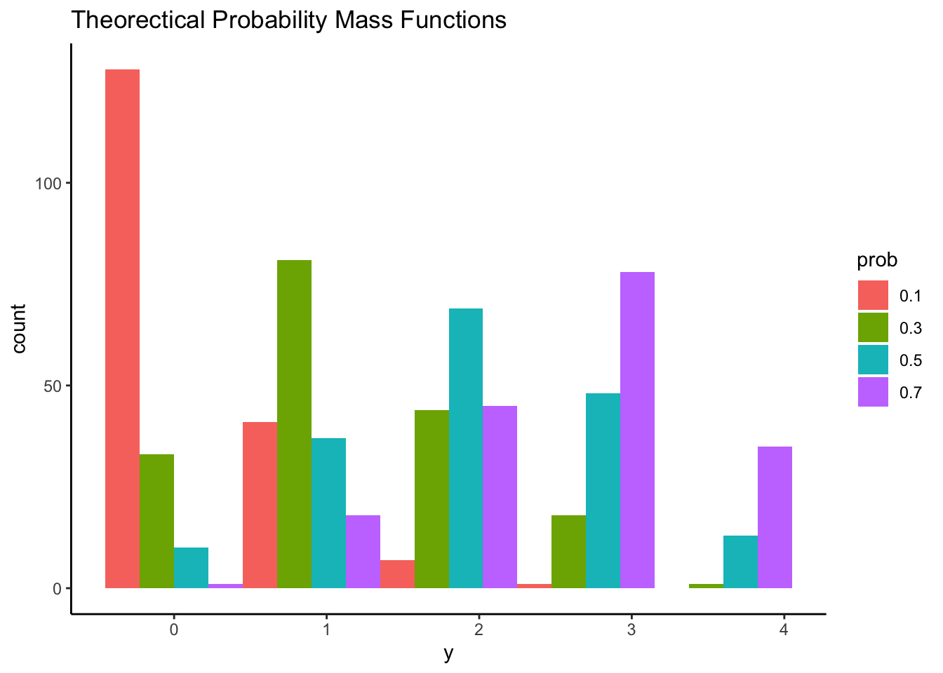
Fixing n = 4 and probability of “brief in conspiracy theory” for each item p = {.1, .3, .5, .7} , we can know probability mass function across each item response from 0 to 4.
Question: which shape of distribution matches our data’s empirical distribution most?
── Attaching core tidyverse packages ──────────────────────── tidyverse 2.0.0 ──
✔ dplyr     1.1.4     ✔ readr     2.1.5
✔ forcats   1.0.0     ✔ stringr   1.5.1
✔ ggplot2   3.5.1     ✔ tibble    3.2.1
✔ lubridate 1.9.4     ✔ tidyr     1.3.1
✔ purrr     1.0.4
── Conflicts ────────────────────────────────────────── tidyverse_conflicts() ──
✖ dplyr::filter() masks stats::filter()
✖ dplyr::lag()    masks stats::lag()
ℹ Use the conflicted package (<http://conflicted.r-lib.org/>) to force all conflicts to become errors

Attaching package: 'kableExtra'


The following object is masked from 'package:dplyr':

    group_rows


here() starts at /Users/jihong/Documents/Projects/website-jihong

Loading required package: Rcpp

This is blavaan 0.5-8

On multicore systems, we suggest use of future::plan("multicore") or
  future::plan("multisession") for faster post-MCMC computations.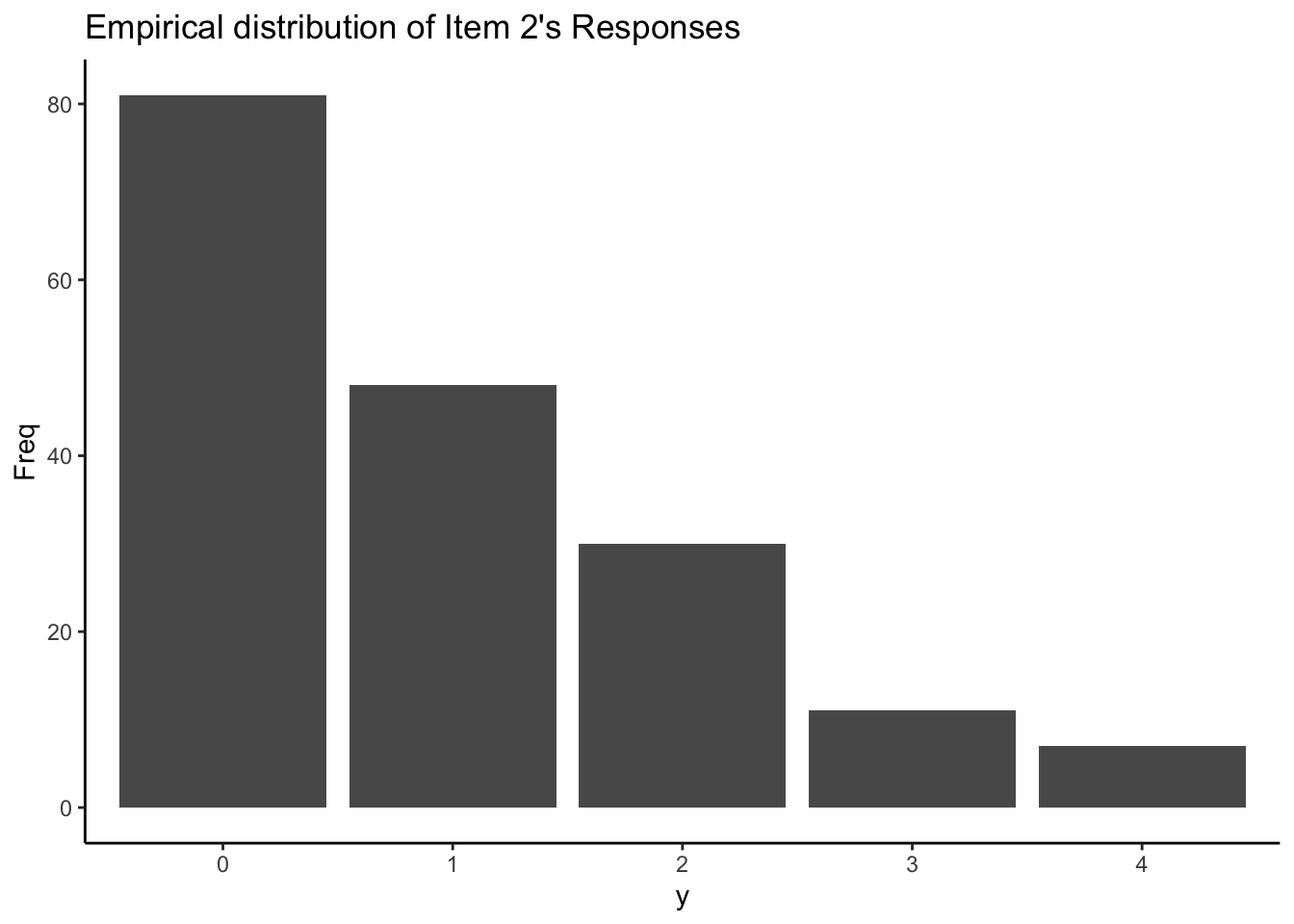
Although it doesn’t seem like our items fit with a binomial, we can actually use this distribution
P(Yi=yi)=(4yi)pyi(1−p)(4−yi)
where probability of success of item i for individual p is as:
ppi=exp(μi+λiθp)1+exp(μi+λiθp)
Note:
The item response model, put into the PDF of the binomial is then:
P(Ypi|θp)=(niYpi)(exp(μi+λiθp)1+exp(μi+λiθp))ypi(1−exp(μi+λiθp)1+exp(μi+λiθp))4−ypi
Further, we can use the same priors as before on each of our item parameters
μi: Normal Prior N(0,100)
λi: Normal prior N(0,100)
Likewise, we can identify the scale of the latent variable as before, too:
model{} for the Binomial Model in Stanmodel {
lambda ~ multi_normal(meanLambda, covLambda); // Prior for item discrimination/factor loadings
mu ~ multi_normal(meanMu, covMu); // Prior for item intercepts
theta ~ normal(0, 1); // Prior for latent variable (with mean/sd specified)
for (item in 1:nItems){
Y[item] ~ binomial(maxItem[item], inv_logit(mu[item] + lambda[item]*theta));
}
}Here, the binomial item response function has two arguments:
maxItem[Item]) is the number of “trials” ni (here, our maximum score minus one – 4)inv_logit(mu[item] + lambda[item]*theta)) is the probability from our model (pi)The data Y[item] must be:
maxItem[item]parameters{} for the Binomial Model in StanNo changes from any of our previous slope/intercept models
data{} for the Binomial Model in Standata {
int<lower=0> nObs; // number of observations
int<lower=0> nItems; // number of items
array[nItems] int<lower=0> maxItem; // maximum value of Item (should be 4 for 5-point Likert)
array[nItems, nObs] int<lower=0> Y; // item responses in an array
vector[nItems] meanMu; // prior mean vector for intercept parameters
matrix[nItems, nItems] covMu; // prior covariance matrix for intercept parameters
vector[nItems] meanLambda; // prior mean vector for discrimination parameters
matrix[nItems, nItems] covLambda; // prior covariance matrix for discrimination parameters
}Note:
Need to supply maxItem (maximum score minus one for each item)
The data are the same (integer) as in the binary/dichotomous item syntax
 0  1  2  3  4
49 51 47 23 7 ### Prepare data list -----------------------------
# data dimensions
nObs = nrow(conspiracyItems)
nItems = ncol(conspiracyItems)
# item intercept hyperparameters
muMeanHyperParameter = 0
muMeanVecHP = rep(muMeanHyperParameter, nItems)
muVarianceHyperParameter = 1000
muCovarianceMatrixHP = diag(x = muVarianceHyperParameter, nrow = nItems)
# item discrimination/factor loading hyperparameters
lambdaMeanHyperParameter = 0
lambdaMeanVecHP = rep(lambdaMeanHyperParameter, nItems)
lambdaVarianceHyperParameter = 1000
lambdaCovarianceMatrixHP = diag(x = lambdaVarianceHyperParameter, nrow = nItems)
modelBinomial_data = list(
nObs = nObs,
nItems = nItems,
maxItem = maxItem,
Y = t(conspiracyItemsBinomial),
meanMu = muMeanVecHP,
covMu = muCovarianceMatrixHP,
meanLambda = lambdaMeanVecHP,
covLambda = lambdaCovarianceMatrixHP
)[1] 1.003589# A tibble: 20 × 10
variable mean median sd mad q5 q95 rhat ess_bulk ess_tail
<chr> <dbl> <dbl> <dbl> <dbl> <dbl> <dbl> <dbl> <dbl> <dbl>
1 mu[1] -0.840 -0.838 0.126 0.126 -1.05 -0.637 1.00 2506. 6240.
2 mu[2] -1.84 -1.83 0.215 0.212 -2.21 -1.50 1.00 2374. 6009.
3 mu[3] -1.99 -1.98 0.223 0.221 -2.38 -1.65 1.00 2662. 6596.
4 mu[4] -1.73 -1.72 0.208 0.206 -2.08 -1.40 1.00 2341. 5991.
5 mu[5] -2.00 -1.99 0.247 0.244 -2.43 -1.62 1.00 2046. 4880.
6 mu[6] -2.10 -2.09 0.241 0.240 -2.51 -1.72 1.00 2370. 6109.
7 mu[7] -2.44 -2.43 0.261 0.257 -2.90 -2.04 1.00 2735. 5943.
8 mu[8] -2.16 -2.15 0.240 0.239 -2.58 -1.79 1.00 2452. 6329.
9 mu[9] -2.40 -2.39 0.278 0.274 -2.88 -1.97 1.00 2412. 6524.
10 mu[10] -3.97 -3.93 0.517 0.511 -4.88 -3.19 1.00 3523. 7434.
11 lambda[1] 1.11 1.10 0.143 0.142 0.881 1.35 1.00 5249. 8927.
12 lambda[2] 1.90 1.89 0.246 0.241 1.53 2.33 1.00 4555. 6779.
13 lambda[3] 1.92 1.90 0.254 0.253 1.52 2.36 1.00 4719. 7465.
14 lambda[4] 1.89 1.88 0.235 0.230 1.53 2.30 1.00 4539. 7441.
15 lambda[5] 2.28 2.26 0.281 0.277 1.84 2.76 1.00 4041. 7534.
16 lambda[6] 2.15 2.13 0.273 0.269 1.72 2.62 1.00 4082. 6668.
17 lambda[7] 2.13 2.11 0.293 0.292 1.68 2.64 1.00 4389. 6712.
18 lambda[8] 2.08 2.07 0.268 0.263 1.67 2.55 1.00 4109. 6184.
19 lambda[9] 2.35 2.33 0.315 0.308 1.87 2.90 1.00 4302. 7267.
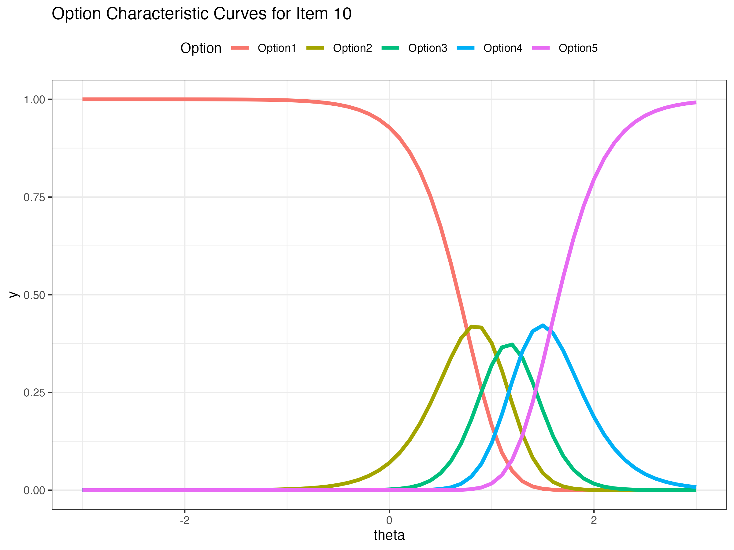
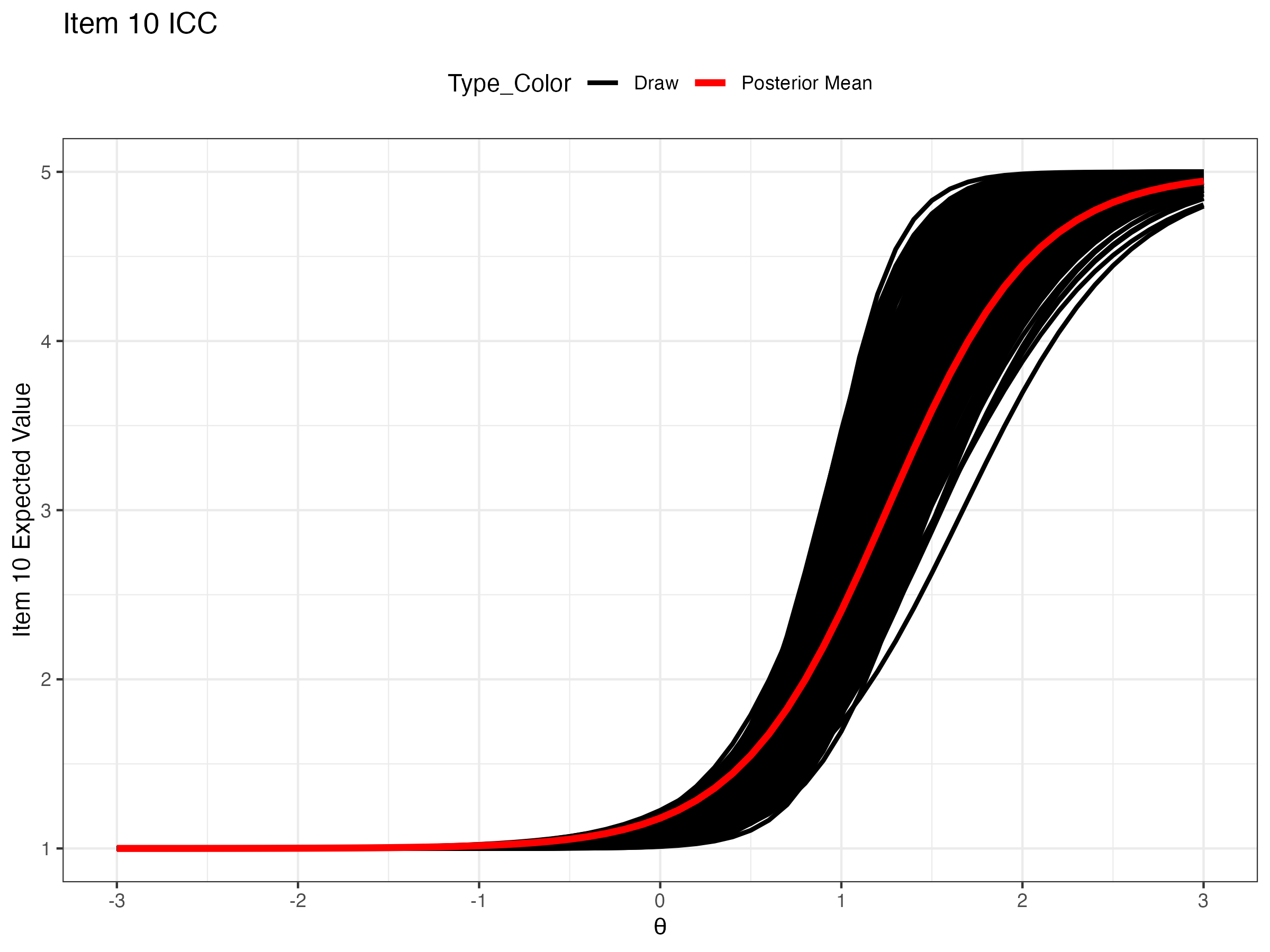
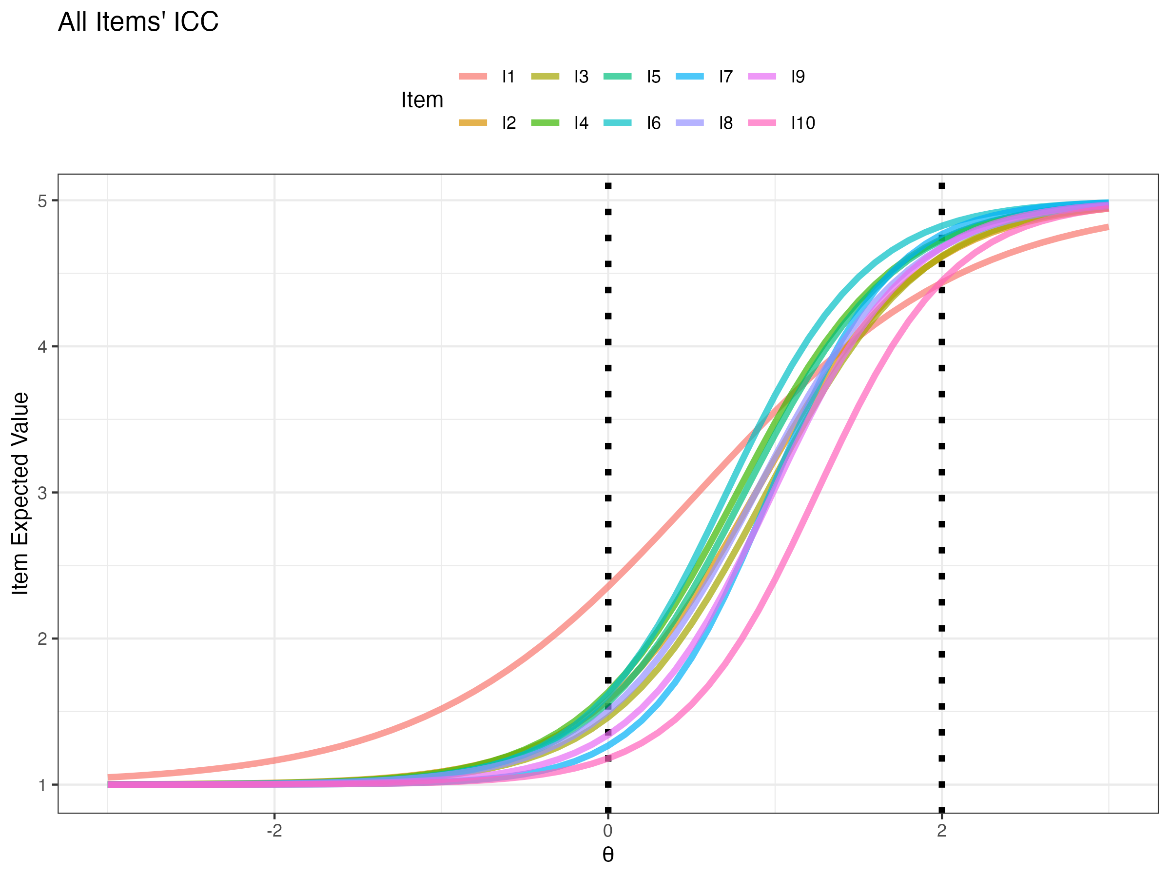
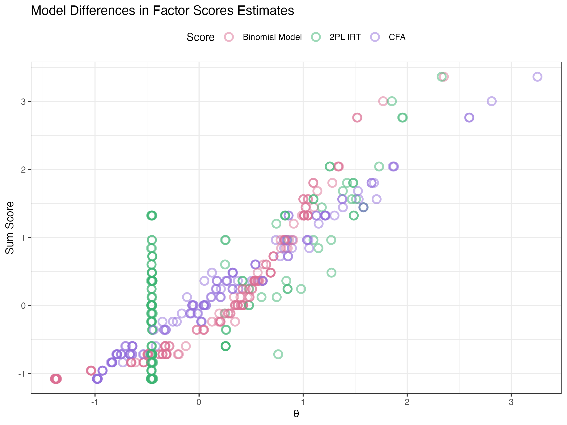
20 lambda[10] 3.40 3.36 0.559 0.541 2.56 4.39 1.00 4807. 6536.Expected probability of certain response across a range of latent variable θ
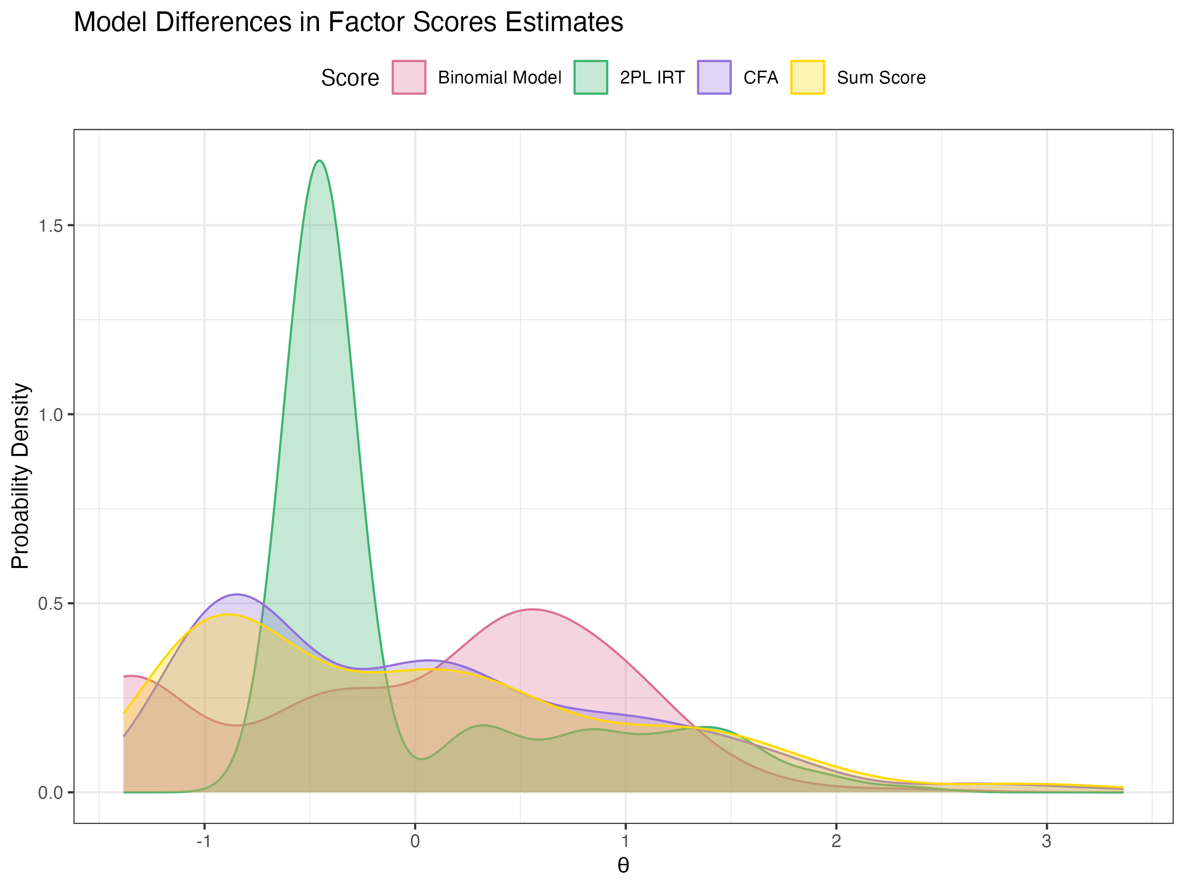
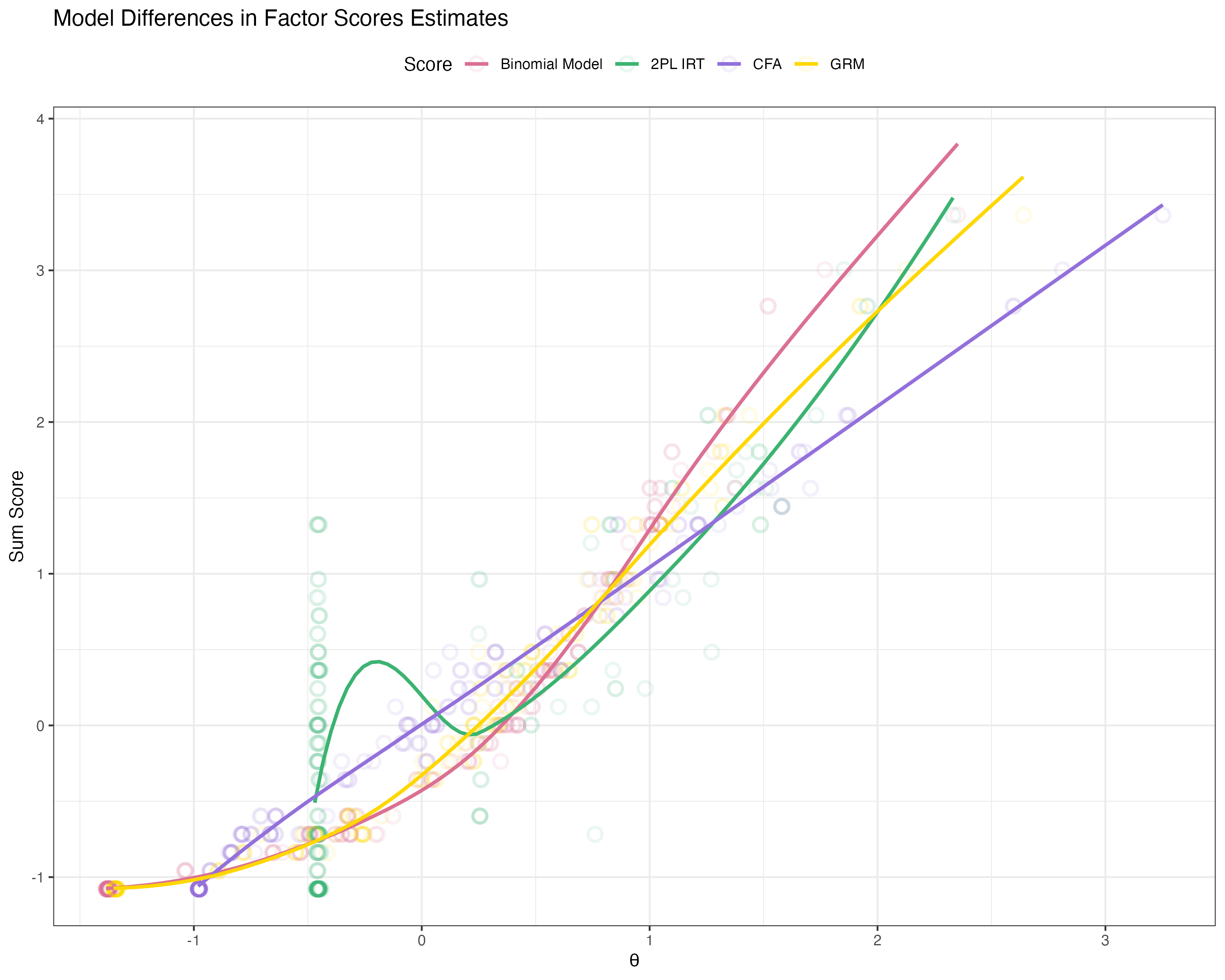
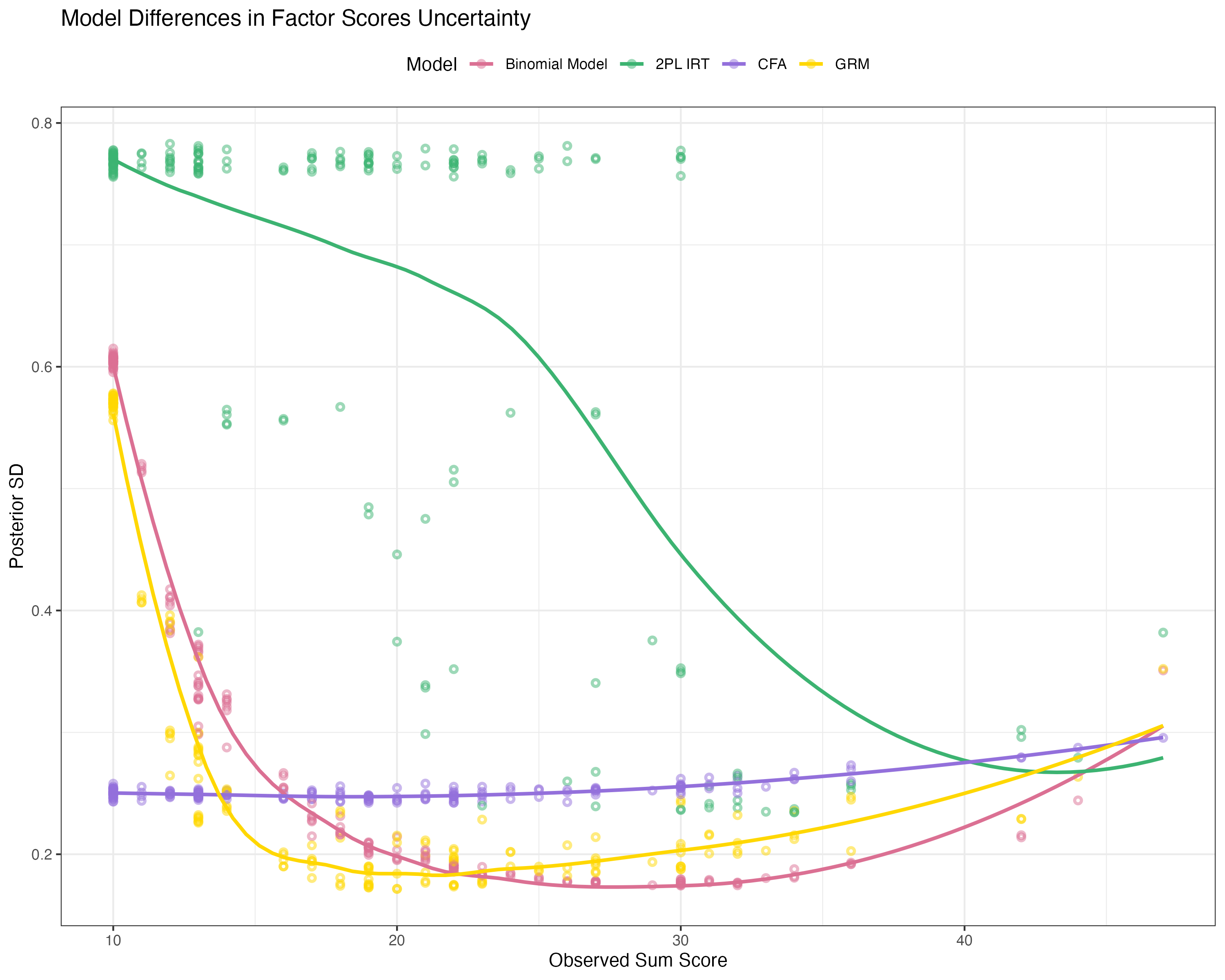
Compare factors scores of Binomial model to 2PL-IRT
Although the binomial distribution is easy, it may not fit our data well
P(Y=y)=n!yi!…yC!py11…pyCC
Here,
n: number of “trials”
yc: number of events in each of c categories (c ∈{1,⋯,C}; Σcyc=n)
pc: probability of observing an event in category c
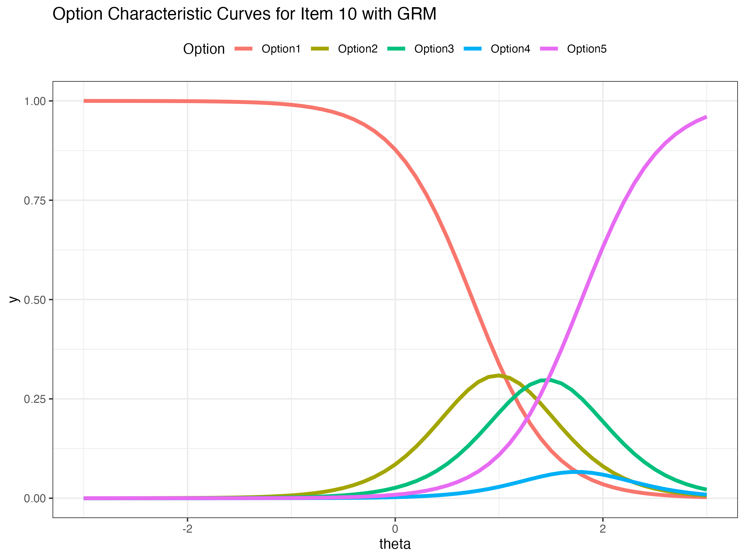
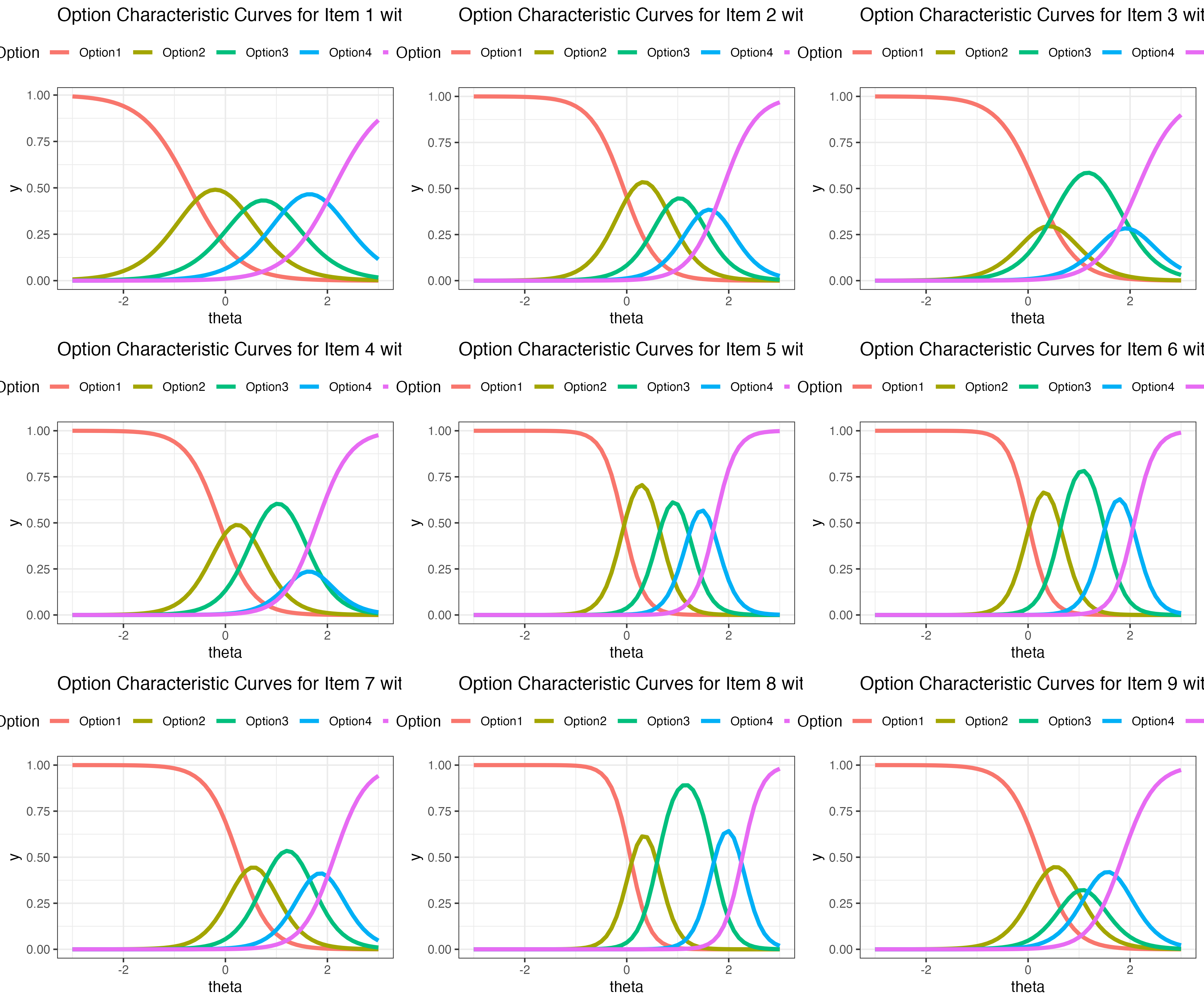
GRM is one of the most popular model for ordered categorical response
P(Yic|θ)=1−P∗(Yi1|θ) if c=1P(Yic|θ)=P∗(Yi,c−1|θ)−P∗(Yi,c|θ) if 1<c<CP(Yic|θ)=P∗(Yi,C−1|θ) if c=Ciwhere probability of response larger than c:
P∗(Yi,c|θ)=P(Yi,c>c|θ)=exp(μic+λuθp)1+exp(μic+λuθp)
With:
model{} for GRM in Stanmodel {
lambda ~ multi_normal(meanLambda, covLambda); // Prior for item discrimination/factor loadings
theta ~ normal(0, 1); // Prior for latent variable (with mean/sd specified)
for (item in 1:nItems){
thr[item] ~ multi_normal(meanThr[item], covThr[item]); // Prior for item intercepts
Y[item] ~ ordered_logistic(lambda[item]*theta, thr[item]);
}
}ordered_logistic is the built-in Stan function for ordered categorical outcomes
Two arguments neeeded for the function
lambda[item]*theta is the muliplications
thr[item] is the thresholds for the item, which is negative values of item intercept
The function expects the response of Y starts from 1
parameters{} for GRM in StanNote that we need to declare threshould as: ordered[maxCategory-1] so that
τi1<τi2<⋯<τiC−1
data{} for GRM in Standata {
int<lower=0> nObs; // number of observations
int<lower=0> nItems; // number of items
int<lower=0> maxCategory;
array[nItems, nObs] int<lower=1, upper=5> Y; // item responses in an array
array[nItems] vector[maxCategory-1] meanThr; // prior mean vector for intercept parameters
array[nItems] matrix[maxCategory-1, maxCategory-1] covThr; // prior covariance matrix for intercept parameters
vector[nItems] meanLambda; // prior mean vector for discrimination parameters
matrix[nItems, nItems] covLambda; // prior covariance matrix for discrimination parameters
}Note that the input for the prior mean/covariance matrix for threshold parameters is now an array (one mean vector and covariance matrix per item)
To match the array for input for the threshold hyperparameter matrices, a little data manipulation is needed
# item threshold hyperparameters
thrMeanHyperParameter = 0
thrMeanVecHP = rep(thrMeanHyperParameter, maxCategory-1)
thrMeanMatrix = NULL
for (item in 1:nItems){
  thrMeanMatrix = rbind(thrMeanMatrix, thrMeanVecHP)
}

thrVarianceHyperParameter = 1000
thrCovarianceMatrixHP = diag(x = thrVarianceHyperParameter, nrow = maxCategory-1)
thrCovArray = array(data = 0, dim = c(nItems, maxCategory-1, maxCategory-1))
for (item in 1:nItems){
  thrCovArray[item, , ] = diag(x = thrVarianceHyperParameter, nrow = maxCategory-1)
}
R array matches Stan’s array type
[1] 1.003504# A tibble: 50 × 10
variable mean median sd mad q5 q95 rhat ess_bulk
<chr> <dbl> <dbl> <dbl> <dbl> <dbl> <dbl> <dbl> <dbl>
1 lambda[1] 2.13 2.11 0.286 0.282 1.68 2.61 1.00 4435.
2 lambda[2] 3.06 3.04 0.428 0.422 2.40 3.80 1.00 4504.
3 lambda[3] 2.57 2.55 0.382 0.376 1.98 3.23 1.00 5053.
4 lambda[4] 3.09 3.07 0.423 0.416 2.44 3.82 1.00 4762.
5 lambda[5] 4.98 4.92 0.762 0.746 3.84 6.34 1.00 3883.
6 lambda[6] 5.01 4.95 0.760 0.738 3.88 6.35 1.00 4065.
7 lambda[7] 3.22 3.19 0.487 0.483 2.47 4.06 1.00 4260.
8 lambda[8] 5.33 5.26 0.863 0.839 4.06 6.87 1.00 3751.
9 lambda[9] 3.14 3.10 0.480 0.472 2.40 3.97 1.00 4633.
10 lambda[10] 2.64 2.61 0.473 0.463 1.92 3.47 1.00 5129.
11 mu[1,1] 1.49 1.48 0.286 0.285 1.03 1.97 1.00 2189.
12 mu[2,1] 0.182 0.185 0.332 0.325 -0.374 0.712 1.00 1430.
13 mu[3,1] -0.447 -0.442 0.297 0.296 -0.944 0.0271 1.00 1641.
14 mu[4,1] 0.348 0.350 0.336 0.334 -0.204 0.895 1.00 1427.
15 mu[5,1] 0.332 0.338 0.494 0.483 -0.484 1.14 1.00 1188.
16 mu[6,1] -0.0321 -0.0198 0.498 0.488 -0.859 0.769 1.00 1166.
17 mu[7,1] -0.809 -0.793 0.360 0.353 -1.42 -0.245 1.00 1424.
18 mu[8,1] -0.381 -0.365 0.530 0.509 -1.28 0.454 1.00 1187.
19 mu[9,1] -0.740 -0.726 0.353 0.346 -1.34 -0.185 1.00 1487.
20 mu[10,1] -1.97 -1.95 0.394 0.385 -2.65 -1.37 1.00 2329.
21 mu[1,2] -0.654 -0.649 0.258 0.256 -1.09 -0.244 1.00 1816.
22 mu[2,2] -2.21 -2.19 0.390 0.381 -2.88 -1.61 1.00 1918.
23 mu[3,2] -1.67 -1.66 0.327 0.321 -2.23 -1.15 1.00 1901.
24 mu[4,2] -1.79 -1.78 0.366 0.361 -2.42 -1.22 1.00 1668.
25 mu[5,2] -3.18 -3.14 0.627 0.608 -4.28 -2.23 1.00 1807.
26 mu[6,2] -3.25 -3.21 0.612 0.599 -4.30 -2.31 1.00 1660.
27 mu[7,2] -2.72 -2.71 0.435 0.425 -3.48 -2.04 1.00 1879.
28 mu[8,2] -3.26 -3.22 0.649 0.637 -4.41 -2.29 1.00 1655.
29 mu[9,2] -2.67 -2.64 0.433 0.424 -3.42 -1.99 1.00 2109.
30 mu[10,2] -3.25 -3.22 0.463 0.455 -4.05 -2.54 1.00 2987.
31 mu[1,3] -2.51 -2.50 0.317 0.319 -3.04 -2.00 1.00 2449.
32 mu[2,3] -4.13 -4.11 0.500 0.494 -5.00 -3.36 1.00 3009.
33 mu[3,3] -4.35 -4.32 0.517 0.503 -5.26 -3.56 1.00 4073.
34 mu[4,3] -4.59 -4.56 0.538 0.533 -5.52 -3.75 1.00 3361.
35 mu[5,3] -6.04 -5.98 0.867 0.852 -7.56 -4.73 1.00 3042.
36 mu[6,3] -7.47 -7.39 1.02 1.00 -9.25 -5.93 1.00 3599.
37 mu[7,3] -5.11 -5.08 0.636 0.629 -6.21 -4.12 1.00 3421.
38 mu[8,3] -9.02 -8.89 1.32 1.29 -11.4 -7.07 1.00 4280.
39 mu[9,3] -4.00 -3.98 0.521 0.512 -4.90 -3.19 1.00 2803.
40 mu[10,3] -4.48 -4.44 0.560 0.551 -5.45 -3.62 1.00 4067.
41 mu[1,4] -4.53 -4.50 0.507 0.506 -5.39 -3.74 1.00 5718.
42 mu[2,4] -5.76 -5.72 0.683 0.676 -6.94 -4.69 1.00 5189.
43 mu[3,4] -5.52 -5.48 0.660 0.649 -6.67 -4.50 1.00 5692.
44 mu[4,4] -5.55 -5.52 0.635 0.623 -6.65 -4.57 1.00 4458.
45 mu[5,4] -8.62 -8.53 1.17 1.14 -10.7 -6.85 1.00 4420.
46 mu[6,4] -10.4 -10.3 1.46 1.44 -13.0 -8.23 1.00 6549.
47 mu[7,4] -6.87 -6.81 0.871 0.851 -8.36 -5.52 1.00 5615.
48 mu[8,4] -12.1 -11.9 1.91 1.86 -15.5 -9.26 1.00 7019.
49 mu[9,4] -5.79 -5.75 0.714 0.703 -7.04 -4.70 1.00 4707.
50 mu[10,4] -4.74 -4.71 0.589 0.583 -5.77 -3.83 1.00 4319.
# ℹ 1 more variable: ess_tail <dbl>