Lecture 11
Multidimensionality and Missing Data
Multidimensionality and Missing Data
Educational Statistics and Research Methods
The course evaluation will be open on April 23 and end on May 3. It is important for me. Please make sure fill out the survey.
We need to create latent variables by specifying which items measure which latent variables in an analysis model
This procedure Called different names by different fields:
Alignment (education measurement)
Factor pattern matrix (factor analysis)
Q-matrix (Question matrix; diagnostic models and multidimensional IRT)
The alignment provides a specification of which latent variables are measured by which items
The math definition of either of these terms is simply whether or not a latent variable appears as a predictor for an item
For instance, item one appears to measure nongovernment conspiracies, meaning its alignment (row vector of the Q-matrix)
The model for the first item is then built with only the factors measured by the item as being present:
f(E(Yp1|θp)=μ1+0∗λ11θp1+1∗λ21θp2=μ1+λ21θp2
Where:
μ1 is the item intercept
λ11 is the factor loading for item 1 (the first subscript) loaded on factor 1 (the second subscript)
θp1 is the value of the latent variable for person p and factor 1
The second factor is not included in the model for the item
If item 1 is only measured by NonGov, we can map item responses to factor loadings and theta via Q-matrix
f(E(Yp1|θp)=μ1+q11(λ11θp1)+q12(λ12θp2)=μ1+θpdiag(q)λ1=μ1+[θp1 θp2][0 00 1][λ11λ12]=μ1+[θp1 θp2][0λ12]=μ1+λ12θp2
Where:
λ1 = [λ11λ12] contains all possible factor loadings for item 1 (size 2 × 1)
θp=[θp1 θp2] contains the factor scores for person p
diag(qi)=qi[1 00 1]=[0 1][1 00 1]=[0 00 1] is a diagonal matrix of ones times the vector of Q-matrix entries for item 1.
Given the Q-matrix each item has its own model using the alignment specifications.
f(E(Yp1|θp))=μ1+λ12θp2f(E(Yp2|θp))=μ1+λ21θp1⋯f(E(Yp10|θp))=μ1+λ10,1θp10
GRM is one of the most popular model for ordered categorical response
P(Yic|θ)=1−P∗(Yi1|θ) if c=1P(Yic|θ)=P∗(Yi,c−1|θ)−P∗(Yi,c|θ) if 1<c<CiP(Yic|θ)=P∗(Yi,C−1|θ) if c=Ciwhere probability of response larger than c:
P∗(Yi,c|θ)=P(Yi,c>c|θ)=exp(μic+λijθpj)1+exp(μic+λijθpj)
With:
Stan, we model item thresholds (difficulty) τc =μc, so that τ1<τ2<⋯<τCi−1parameters {
array[nObs] vector[nFactors] theta; // the latent variables (one for each person)
array[nItems] ordered[maxCategory-1] thr; // the item thresholds (one for each item category minus one)
vector[nLoadings] lambda; // the factor loadings/item discriminations (one for each item)
cholesky_factor_corr[nFactors] thetaCorrL;
}Note:
theta is a array (for the MVN prior)thr is the same as the unidimensional modellambda is the vector of all factor loadings to be estimated (needs nLoadings)thetaCorrL is of type chelesky_factor_corr, a built in type that identifies this as lower diagonal of a Cholesky-factorized correlation matrixtransformed data{
int<lower=0> nLoadings = 0; // number of loadings in model
for (factor in 1:nFactors){
nLoadings = nLoadings + sum(Qmatrix[1:nItems, factor]); // Total number of loadings to be estimated
}
array[nLoadings, 2] int loadingLocation; // the row/column positions of each loading
int loadingNum=1;
for (item in 1:nItems){
for (factor in 1:nFactors){
if (Qmatrix[item, factor] == 1){
loadingLocation[loadingNum, 1] = item;
loadingLocation[loadingNum, 2] = factor;
loadingNum = loadingNum + 1;
}
}
}
}Note:
transformed data {} block runs prior to the Markov Chain;
nLoadings
Stan the row and column position of each loading in loadingMatrix used in the model {} blocktransformed parameters{
matrix[nItems, nFactors] lambdaMatrix = rep_matrix(0.0, nItems, nFactors);
matrix[nObs, nFactors] thetaMatrix;
// build matrix for lambdas to multiply theta matrix
for (loading in 1:nLoadings){
lambdaMatrix[loadingLocation[loading,1], loadingLocation[loading,2]] = lambda[loading];
}
for (factor in 1:nFactors){
thetaMatrix[,factor] = to_vector(theta[,factor]);
}
}Note:
transformed parameters {} block runs prior to each iteration of the Markov chain
thetaMatrix (converting theta from an array to a matrix)lambdaMatrix (puts the loadings and zeros from the Q-matrix into correct position)
lambdaMatrix initialized at zero so we just have to add the loadings in the correct positionmodel {
lambda ~ multi_normal(meanLambda, covLambda);
thetaCorrL ~ lkj_corr_cholesky(1.0);
theta ~ multi_normal_cholesky(meanTheta, thetaCorrL);
for (item in 1:nItems){
thr[item] ~ multi_normal(meanThr[item], covThr[item]);
Y[item] ~ ordered_logistic(thetaMatrix*lambdaMatrix[item,1:nFactors]', thr[item]);
}
}thetaMatrix is a matrix of latent variables for each person with N×J. Generated by MVN with factor mean and factor covaraince
Θ∼MVM(μΘ,ΣΘ)
We need to convert theta from array to a matrix in transformed parameters block.
From Q matrix to loading location matrix Loc
Q=[0 11 00 10 11 00 11 01 01 01 1]Loc=[1 22 13 24 25 16 27 18 19 110 110 2]
Λ[Loc[j,1],Loc[j,2]]=λjkΛ=[0 .3.5 00 .50 .3.7 00 .5.2 0.7 0.8 0.3 .2]
Where j denotes the index of lambda.
model {
  lambda ~ multi_normal(meanLambda, covLambda);
  thetaCorrL ~ lkj_corr_cholesky(1.0);
  theta ~ multi_normal_cholesky(meanTheta, thetaCorrL);

  for (item in 1:nItems){
    thr[item] ~ multi_normal(meanThr[item], covThr[item]);
    Y[item] ~ ordered_logistic(thetaMatrix*lambdaMatrix[item,1:nFactors]', thr[item]);
  }
}transformed data{
int<lower=0> nLoadings = 0; // number of loadings in model
for (factor in 1:nFactors){
nLoadings = nLoadings + sum(Qmatrix[1:nItems, factor]);
}
array[nLoadings, 2] int loadingLocation; // the row/column positions of each loading
int loadingNum=1;
for (item in 1:nItems){
for (factor in 1:nFactors){
if (Qmatrix[item, factor] == 1){
loadingLocation[loadingNum, 1] = item;
loadingLocation[loadingNum, 2] = factor;
loadingNum = loadingNum + 1;
}
}
}
}loadingLocation with first column as item index and second column as factor index;lambdaMatrix puts the proposed loadings and zeros from the Q-matrix into correct positiondata {
// data specifications =============================================================
int<lower=0> nObs; // number of observations
int<lower=0> nItems; // number of items
int<lower=0> maxCategory; // number of categories for each item
// input data =============================================================
array[nItems, nObs] int<lower=1, upper=5> Y; // item responses in an array
// loading specifications =============================================================
int<lower=1> nFactors; // number of loadings in the model
array[nItems, nFactors] int<lower=0, upper=1> Qmatrix;
// prior specifications =============================================================
array[nItems] vector[maxCategory-1] meanThr; // prior mean vector for intercept parameters
array[nItems] matrix[maxCategory-1, maxCategory-1] covThr; // prior covariance matrix for intercept parameters
vector[nItems] meanLambda; // prior mean vector for discrimination parameters
matrix[nItems, nItems] covLambda; // prior covariance matrix for discrimination parameters
vector[nFactors] meanTheta;
}Note:
meanTheta: Factor means (hyperparameters) are added (but we will set these to zero)nFactors: Number of latent variables (needed for Q-matrix)Qmatrix: Q-matrix for modelNote:
Converts thresholds to intercepts mu
Creates thetaCorr by multiplying Cholesky-factor lower triangle with upper triangle
thetaCorr when looking at model outputWe run Stan the same way we have previously:
here() starts at /Users/jihong/Documents/Projects/website-jihongWarning: package 'cmdstanr' was built under R version 4.4.3This is cmdstanr version 0.8.1- CmdStanR documentation and vignettes: mc-stan.org/cmdstanr- CmdStan path: /Users/jihong/.cmdstan/cmdstan-2.36.0- CmdStan version: 2.36.0Note:
[1] 1.082978# A tibble: 54 × 10
variable mean median sd mad q5 q95 rhat ess_bulk
<chr> <dbl> <dbl> <dbl> <dbl> <dbl> <dbl> <dbl> <dbl>
1 lambda[1] 2.00 1.99 0.265 0.259 1.59 2.46 1.00 3041.
2 lambda[2] 2.84 2.82 0.382 0.372 2.25 3.51 1.00 2718.
3 lambda[3] 2.40 2.38 0.342 0.338 1.87 2.99 1.00 3657.
4 lambda[4] 2.93 2.90 0.389 0.380 2.32 3.60 1.00 3332.
5 lambda[5] 4.34 4.30 0.597 0.606 3.41 5.38 1.00 2542.
6 lambda[6] 4.23 4.20 0.570 0.560 3.36 5.23 1.00 2611.
7 lambda[7] 2.86 2.84 0.410 0.402 2.24 3.57 1.00 3546.
8 lambda[8] 4.14 4.10 0.566 0.552 3.26 5.12 1.00 2429.
9 lambda[9] 2.91 2.89 0.423 0.421 2.25 3.64 1.00 3071.
10 lambda[10] 2.45 2.42 0.429 0.417 1.80 3.19 1.00 4312.
11 mu[1,1] 1.88 1.87 0.291 0.292 1.42 2.37 1.00 1552.
12 mu[2,1] 0.819 0.811 0.304 0.302 0.325 1.33 1.01 864.
13 mu[3,1] 0.0995 0.102 0.263 0.260 -0.328 0.530 1.01 1005.
14 mu[4,1] 0.998 0.991 0.320 0.317 0.490 1.53 1.00 893.
15 mu[5,1] 1.32 1.31 0.430 0.421 0.641 2.05 1.01 729.
16 mu[6,1] 0.973 0.966 0.418 0.406 0.305 1.67 1.01 741.
17 mu[7,1] -0.103 -0.103 0.293 0.289 -0.578 0.376 1.01 877.
18 mu[8,1] 0.704 0.697 0.397 0.388 0.0702 1.37 1.01 760.
19 mu[9,1] -0.0561 -0.0587 0.297 0.294 -0.540 0.435 1.00 877.
20 mu[10,1] -1.36 -1.35 0.310 0.304 -1.89 -0.869 1.00 1370.
21 mu[1,2] -0.209 -0.206 0.235 0.229 -0.602 0.172 1.00 1015.
22 mu[2,2] -1.52 -1.51 0.320 0.321 -2.05 -1.01 1.00 1106.
23 mu[3,2] -1.10 -1.10 0.276 0.270 -1.56 -0.662 1.00 1075.
24 mu[4,2] -1.14 -1.13 0.312 0.311 -1.66 -0.637 1.00 940.
25 mu[5,2] -1.95 -1.94 0.451 0.438 -2.72 -1.24 1.00 974.
26 mu[6,2] -1.99 -1.98 0.431 0.428 -2.72 -1.30 1.01 947.
27 mu[7,2] -1.95 -1.94 0.341 0.336 -2.54 -1.41 1.00 1167.
28 mu[8,2] -1.82 -1.81 0.418 0.412 -2.54 -1.17 1.01 900.
29 mu[9,2] -1.95 -1.93 0.346 0.339 -2.53 -1.40 1.00 1251.
30 mu[10,2] -2.60 -2.58 0.368 0.371 -3.23 -2.02 1.00 1954.
31 mu[1,3] -2.03 -2.02 0.281 0.283 -2.50 -1.58 1.00 1398.
32 mu[2,3] -3.38 -3.36 0.412 0.409 -4.09 -2.74 1.00 1855.
33 mu[3,3] -3.68 -3.66 0.437 0.433 -4.43 -3.00 1.00 2948.
34 mu[4,3] -3.85 -3.83 0.456 0.448 -4.64 -3.13 1.00 1934.
35 mu[5,3] -4.56 -4.53 0.606 0.589 -5.62 -3.61 1.00 2031.
36 mu[6,3] -5.61 -5.59 0.675 0.682 -6.75 -4.55 1.00 2530.
37 mu[7,3] -4.14 -4.13 0.505 0.503 -5.01 -3.35 1.00 2298.
38 mu[8,3] -6.41 -6.37 0.777 0.766 -7.77 -5.20 1.00 3221.
39 mu[9,3] -3.24 -3.23 0.422 0.423 -3.96 -2.58 1.00 1797.
40 mu[10,3] -3.76 -3.74 0.451 0.450 -4.54 -3.04 1.00 2814.
41 mu[1,4] -3.98 -3.95 0.454 0.448 -4.76 -3.27 1.00 3838.
42 mu[2,4] -4.91 -4.88 0.573 0.568 -5.90 -4.02 1.00 3794.
43 mu[3,4] -4.76 -4.74 0.561 0.558 -5.73 -3.90 1.00 4789.
44 mu[4,4] -4.75 -4.73 0.548 0.542 -5.69 -3.90 1.00 2753.
45 mu[5,4] -6.83 -6.78 0.848 0.849 -8.31 -5.52 1.00 3543.
46 mu[6,4] -7.93 -7.88 0.976 0.974 -9.62 -6.40 1.00 5887.
47 mu[7,4] -5.70 -5.66 0.698 0.702 -6.91 -4.63 1.00 3865.
48 mu[8,4] -8.48 -8.43 1.10 1.07 -10.4 -6.78 1.00 6211.
49 mu[9,4] -4.95 -4.91 0.595 0.588 -5.98 -4.03 1.00 3195.
50 mu[10,4] -4.01 -3.99 0.477 0.472 -4.84 -3.27 1.00 3214.
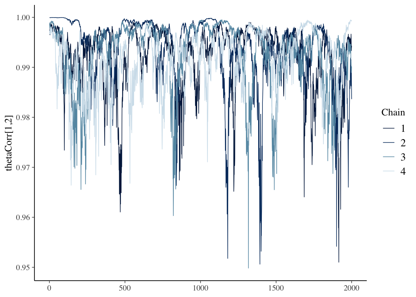
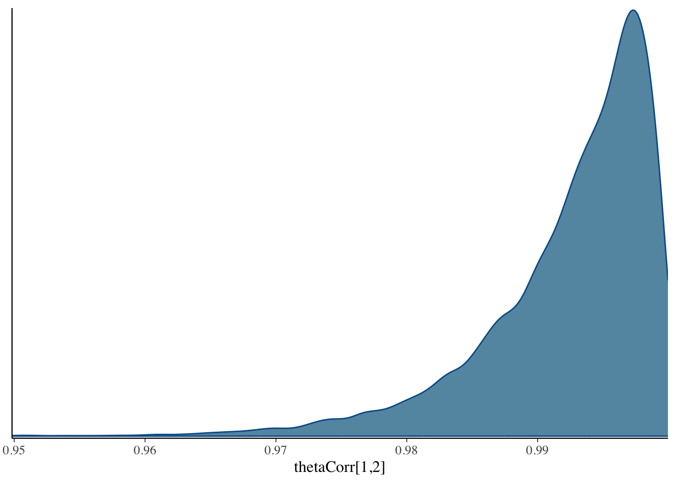
51 thetaCorr[1,1] 1 1 0 0 1 1 NA NA
52 thetaCorr[2,1] 0.992 0.994 0.00650 0.00499 0.979 0.999 1.08 41.2
53 thetaCorr[1,2] 0.992 0.994 0.00650 0.00499 0.979 0.999 1.08 41.2
54 thetaCorr[2,2] 1 1 0 0 1 1 NA NA
# ℹ 1 more variable: ess_tail <dbl>Lambda_postmean <- modelOrderedLogit_samples$summary(variables = "lambda", .cores = 5)$mean
Q = matrix(c(
0, 1,
1, 0,
0, 1,
0, 1,
1, 0,
0, 1,
1, 0,
1, 0,
1, 0,
0, 1), ncol=2, byrow = T)
Lambda_mat <- Q
i = 0
for (r in 1:nrow(Q)) {
for (c in 1:ncol(Q)) {
if (Q[r, c]) {
i = i + 1
Lambda_mat[r, c] <- Lambda_postmean[i]
}
}
}
colnames(Lambda_mat) <- c("F1", "F2")
rownames(Lambda_mat) <- paste0("Item", 1:10)
Lambda_mat F1 F2
Item1 0.000000 2.004086
Item2 2.839446 0.000000
Item3 0.000000 2.400975
Item4 0.000000 2.925028
Item5 4.337551 0.000000
Item6 0.000000 4.228389
Item7 2.861449 0.000000
Item8 4.138962 0.000000
Item9 2.911422 0.000000
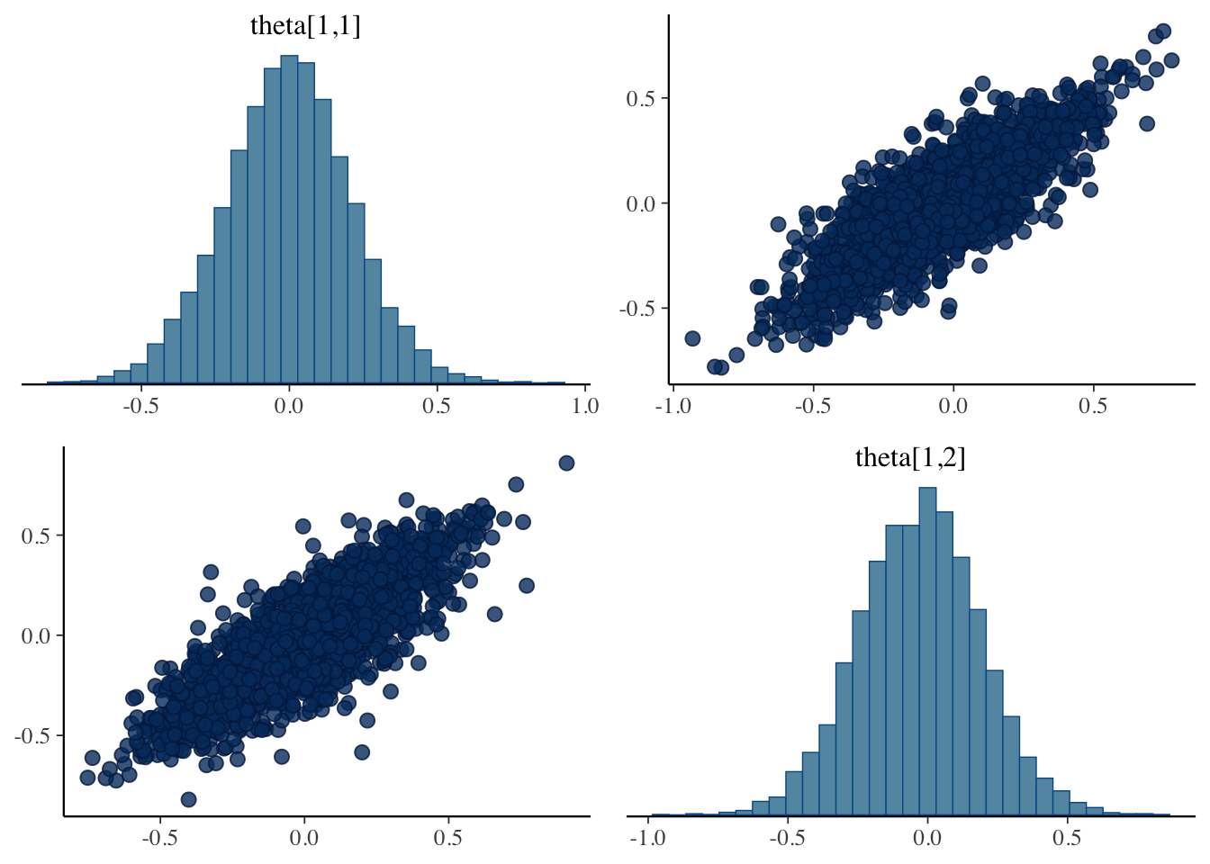
Item10 0.000000 2.447148This is bayesplot version 1.11.1- Online documentation and vignettes at mc-stan.org/bayesplot- bayesplot theme set to bayesplot::theme_default() * Does _not_ affect other ggplot2 plots * See ?bayesplot_theme_set for details on theme settingPlots of draws from person 1
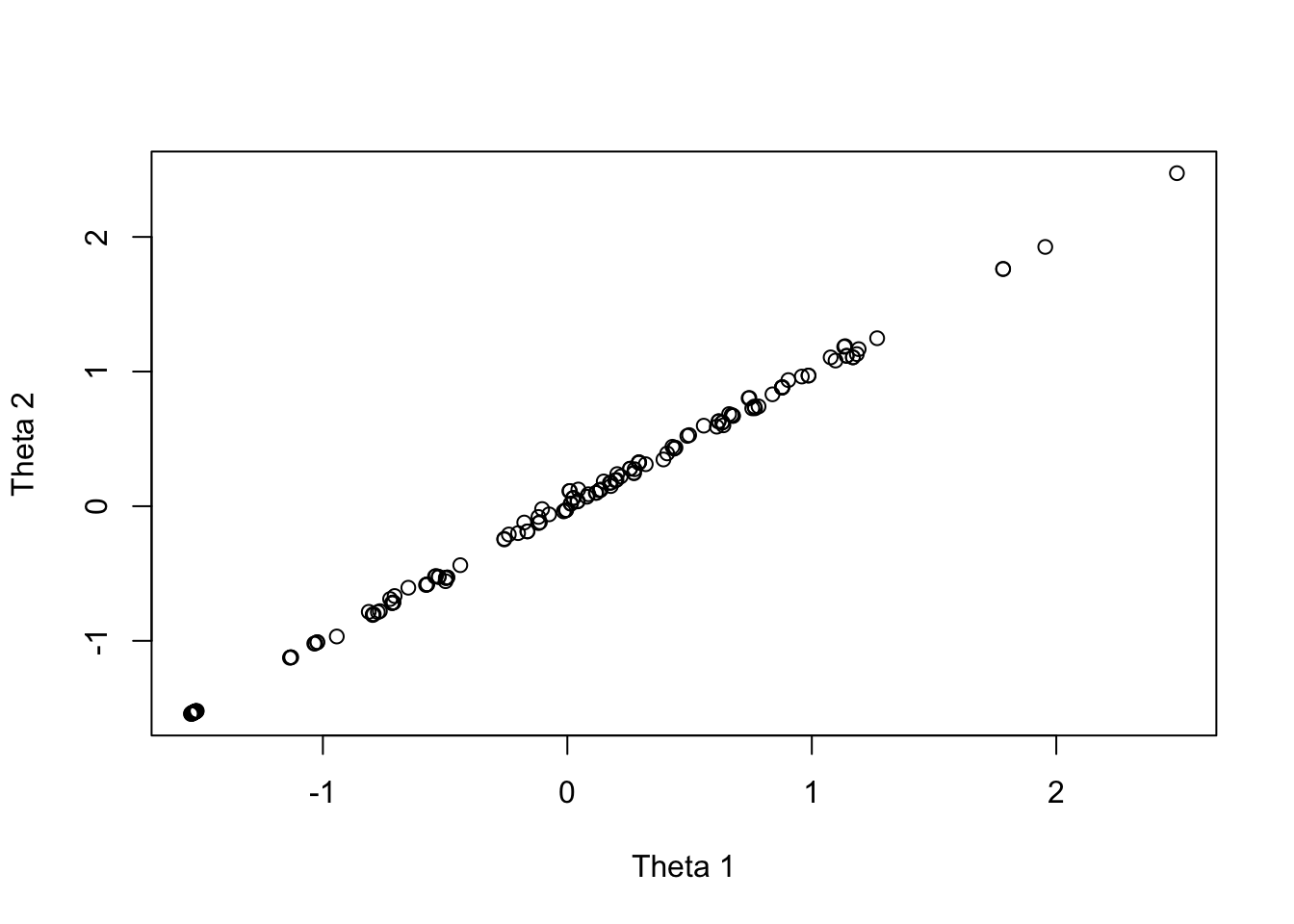
Relationships of sample EAP of Factor 1 and Factor 2
If you ever attempted to analyze missing data in Stan, you likely received an error message:
Error: Variable 'Y' has NA values.
That is because, by default, Stan does not model missing data
Instead, we have to get Stan to work with the data we have (the values that are not missing)
That does not mean remove cases where any observed variables are missing
To make things a bit easier, I’m only turning one value into missing data (the first person’s response to the first item)
Note that all code will work with as missing as you have
We will use the previous syntax with graded response modeling.
The Q-matrix this time will be a single column vector (one dimension)
model {
lambda ~ multi_normal(meanLambda, covLambda);
thetaCorrL ~ lkj_corr_cholesky(1.0);
theta ~ multi_normal_cholesky(meanTheta, thetaCorrL);
for (item in 1:nItems){
thr[item] ~ multi_normal(meanThr[item], covThr[item]);
Y[item, observed[item, 1:nObserved[item]]] ~ ordered_logistic(thetaMatrix[observed[item, 1:nObserved[item]],]*lambdaMatrix[item,1:nFactors]', thr[item]);
}
}Notes:
Big change is in Y:
Previous: Y[item]
Now: Y[item, observed[item,1:nObserveed[item]]]
Mirroring this is a change to thetaMatrix[observed[item, 1:nObserved[item]],]
data {
// data specifications =============================================================
int<lower=0> nObs; // number of observations
int<lower=0> nItems; // number of items
int<lower=0> maxCategory; // number of categories for each item
array[nItems] int nObserved;
array[nItems, nObs] array[nItems] int observed;
// input data =============================================================
array[nItems, nObs] int<lower=-1, upper=5> Y; // item responses in an array
// loading specifications =============================================================
int<lower=1> nFactors; // number of loadings in the model
array[nItems, nFactors] int<lower=0, upper=1> Qmatrix;
// prior specifications =============================================================
array[nItems] vector[maxCategory-1] meanThr; // prior mean vector for intercept parameters
array[nItems] matrix[maxCategory-1, maxCategory-1] covThr; // prior covariance matrix for intercept parameters
vector[nItems] meanLambda; // prior mean vector for discrimination parameters
matrix[nItems, nItems] covLambda; // prior covariance matrix for discrimination parameters
vector[nFactors] meanTheta;
}array[nItems] int Observed : The number of observations with non-missing data for each itemarray[nItems, nObs] array[nItems] int observed : A listing of which observations have non-missing data for each item
To build these arrays, we can use a loop in R:
observed = matrix(data = -1, nrow = nrow(conspiracyItems), ncol = ncol(conspiracyItems))
nObserved = NULL
for (variable in 1:ncol(conspiracyItems)){
nObserved = c(nObserved, length(which(!is.na(conspiracyItems[, variable]))))
observed[1:nObserved[variable], variable] = which(!is.na(conspiracyItems[, variable]))
}For the item that has the first case missing, this gives:
[1] 176 [1] 2 3 4 5 6 7 8 9 10 11 12 13 14 15 16 17 18 19
[19] 20 21 22 23 24 25 26 27 28 29 30 31 32 33 34 35 36 37
[37] 38 39 40 41 42 43 44 45 46 47 48 49 50 51 52 53 54 55
[55] 56 57 58 59 60 61 62 63 64 65 66 67 68 69 70 71 72 73
[73] 74 75 76 77 78 79 80 81 82 83 84 85 86 87 88 89 90 91
[91] 92 93 94 95 96 97 98 99 100 101 102 103 104 105 106 107 108 109
[109] 110 111 112 113 114 115 116 117 118 119 120 121 122 123 124 125 126 127
[127] 128 129 130 131 132 133 134 135 136 137 138 139 140 141 142 143 144 145
[145] 146 147 148 149 150 151 152 153 154 155 156 157 158 159 160 161 162 163
[163] 164 165 166 167 168 169 170 171 172 173 174 175 176 177 -1The item has 176 observed responses and one missing
Entries 1 through 176 of observed[,1] list who has non-missing data
The 177th entry of observed[,1] is -1 (but won’t be used in Stan)
We can use the values of observed[,1] to have Stan only select the corresponding data points that are non-missing
To demonstrate, in R, here is all of the data for the first item
[1] NA 3 4 2 2 1 4 2 3 2 1 3 2 1 2 2 2 2 3 2 1 1 1 1 4
[26] 4 4 3 4 3 3 1 2 1 2 3 1 2 1 2 1 1 2 2 4 3 3 1 1 4
[51] 1 2 1 3 1 1 2 1 4 2 2 2 1 5 3 2 3 3 1 3 2 1 2 1 1
[76] 2 3 4 3 3 2 2 1 3 3 1 2 3 1 4 2 1 2 5 5 2 3 1 3 2
[101] 3 5 2 4 1 3 3 4 3 2 2 4 3 3 4 3 2 2 1 1 3 4 3 2 1
[126] 4 3 2 2 3 4 5 1 5 3 1 3 3 3 2 2 1 1 3 1 3 3 4 1 1
[151] 4 1 4 2 1 1 1 2 2 1 4 2 1 2 4 1 2 5 3 2 1 3 3 3 2
[176] 3 3And here, we select the non-missing using the index values in observed :
[1] 2 3 4 5 6 7 8 9 10 11 12 13 14 15 16 17 18 19
[19] 20 21 22 23 24 25 26 27 28 29 30 31 32 33 34 35 36 37
[37] 38 39 40 41 42 43 44 45 46 47 48 49 50 51 52 53 54 55
[55] 56 57 58 59 60 61 62 63 64 65 66 67 68 69 70 71 72 73
[73] 74 75 76 77 78 79 80 81 82 83 84 85 86 87 88 89 90 91
[91] 92 93 94 95 96 97 98 99 100 101 102 103 104 105 106 107 108 109
[109] 110 111 112 113 114 115 116 117 118 119 120 121 122 123 124 125 126 127
[127] 128 129 130 131 132 133 134 135 136 137 138 139 140 141 142 143 144 145
[145] 146 147 148 149 150 151 152 153 154 155 156 157 158 159 160 161 162 163
[163] 164 165 166 167 168 169 170 171 172 173 174 175 176 177Warning in 1:nObserved: numerical expression has 10 elements: only the first
used [1] 3 4 2 2 1 4 2 3 2 1 3 2 1 2 2 2 2 3 2 1 1 1 1 4 4 4 3 4 3 3 1 2 1 2 3 1 2
[38] 1 2 1 1 2 2 4 3 3 1 1 4 1 2 1 3 1 1 2 1 4 2 2 2 1 5 3 2 3 3 1 3 2 1 2 1 1
[75] 2 3 4 3 3 2 2 1 3 3 1 2 3 1 4 2 1 2 5 5 2 3 1 3 2 3 5 2 4 1 3 3 4 3 2 2 4
[112] 3 3 4 3 2 2 1 1 3 4 3 2 1 4 3 2 2 3 4 5 1 5 3 1 3 3 3 2 2 1 1 3 1 3 3 4 1
[149] 1 4 1 4 2 1 1 1 2 2 1 4 2 1 2 4 1 2 5 3 2 1 3 3 3 2 3 3The values of observed[1:nObserved,1] leads to only using the non-missing data
Finally, we must ensure all data into Stan have no NA values
Dr. Templin’s recommendation: Change all NA values to something that cannot be modeled
-1 here: it cannot be used with ordered_logit() likelihoodThis ensures that Stan won’t model the data by accident
With our missing values denotes, we can run Stan as we have previously
modelOrderedLogit_data = list(
nObs = nObs,
nItems = nItems,
maxCategory = maxCategory,
nObserved = nObserved,
observed = t(observed),
Y = t(Y),
nFactors = ncol(Qmatrix),
Qmatrix = Qmatrix,
meanThr = thrMeanMatrix,
covThr = thrCovArray,
meanLambda = lambdaMeanVecHP,
covLambda = lambdaCovarianceMatrixHP,
meanTheta = thetaMean
)
modelOrderedLogit_samples = modelOrderedLogit_stan$sample(
  data = modelOrderedLogit_data,
  seed = 191120221,
  chains = 4,
  parallel_chains = 4,
  iter_warmup = 2000,
  iter_sampling = 2000,
  init = function() list(lambda=rnorm(nItems, mean=5, sd=1))
)[1] 1.008265# A tibble: 50 × 10
variable mean median sd mad q5 q95 rhat ess_bulk ess_tail
<chr> <dbl> <dbl> <dbl> <dbl> <dbl> <dbl> <dbl> <dbl> <dbl>
1 lambda[1] 2.01 2.00 0.267 0.264 1.59 2.46 1.00 1816. 3503.
2 lambda[2] 2.85 2.83 0.381 0.374 2.26 3.51 1.00 2018. 3514.
3 lambda[3] 2.39 2.37 0.342 0.336 1.86 2.98 1.01 2224. 3805.
4 lambda[4] 2.90 2.88 0.386 0.383 2.31 3.57 1.00 2112. 4057.
5 lambda[5] 4.30 4.26 0.604 0.594 3.38 5.36 1.00 1686. 3370.
6 lambda[6] 4.18 4.15 0.555 0.542 3.32 5.13 1.00 1948. 3628.
7 lambda[7] 2.88 2.86 0.417 0.413 2.24 3.59 1.00 1979. 3752.
8 lambda[8] 4.16 4.13 0.565 0.548 3.30 5.16 1.00 1805. 3518.
9 lambda[9] 2.90 2.87 0.429 0.431 2.24 3.64 1.00 2515. 4050.
10 lambda[1… 2.41 2.39 0.421 0.408 1.76 3.17 1.00 2734. 3889.
11 mu[1,1] 1.87 1.87 0.287 0.286 1.41 2.36 1.00 1328. 2908.
12 mu[2,1] 0.805 0.798 0.304 0.299 0.317 1.32 1.01 698. 1979.
13 mu[3,1] 0.0942 0.0880 0.255 0.249 -0.322 0.525 1.01 855. 2328.
14 mu[4,1] 0.982 0.976 0.309 0.300 0.487 1.50 1.01 825. 2510.
15 mu[5,1] 1.29 1.28 0.418 0.422 0.629 1.98 1.01 545. 1641.
16 mu[6,1] 0.947 0.935 0.392 0.388 0.324 1.61 1.01 651. 2064.
17 mu[7,1] -0.116 -0.115 0.288 0.284 -0.591 0.358 1.01 743. 1984.
18 mu[8,1] 0.680 0.672 0.387 0.380 0.0485 1.33 1.01 536. 1353.
19 mu[9,1] -0.0700 -0.0693 0.295 0.295 -0.560 0.415 1.01 718. 2146.
20 mu[10,1] -1.35 -1.34 0.299 0.294 -1.86 -0.883 1.01 984. 3276.
21 mu[1,2] -0.197 -0.194 0.234 0.231 -0.584 0.191 1.01 1039. 2640.
22 mu[2,2] -1.53 -1.53 0.315 0.311 -2.06 -1.04 1.00 1022. 2850.
23 mu[3,2] -1.10 -1.10 0.270 0.267 -1.56 -0.665 1.00 811. 2432.
24 mu[4,2] -1.13 -1.12 0.308 0.305 -1.65 -0.638 1.01 809. 2367.
25 mu[5,2] -1.95 -1.94 0.434 0.431 -2.68 -1.26 1.00 951. 2479.
26 mu[6,2] -1.97 -1.96 0.419 0.412 -2.68 -1.31 1.01 800. 2150.
27 mu[7,2] -1.96 -1.95 0.336 0.338 -2.54 -1.43 1.00 906. 2466.
28 mu[8,2] -1.84 -1.83 0.408 0.410 -2.53 -1.19 1.01 807. 2086.
29 mu[9,2] -1.95 -1.94 0.339 0.330 -2.52 -1.40 1.01 1076. 2510.
30 mu[10,2] -2.58 -2.57 0.356 0.351 -3.19 -2.03 1.00 1800. 4116.
31 mu[1,3] -2.03 -2.02 0.281 0.280 -2.51 -1.58 1.00 1417. 3411.
32 mu[2,3] -3.40 -3.38 0.402 0.403 -4.08 -2.75 1.00 1660. 3827.
33 mu[3,3] -3.67 -3.66 0.427 0.426 -4.40 -3.00 1.00 2626. 5222.
34 mu[4,3] -3.82 -3.80 0.446 0.442 -4.59 -3.12 1.00 1672. 4166.
35 mu[5,3] -4.53 -4.50 0.585 0.583 -5.53 -3.61 1.00 1842. 3811.
36 mu[6,3] -5.58 -5.54 0.678 0.673 -6.74 -4.54 1.00 1989. 4938.
37 mu[7,3] -4.16 -4.14 0.498 0.493 -5.00 -3.37 1.00 1939. 4002.
38 mu[8,3] -6.43 -6.39 0.776 0.762 -7.79 -5.21 1.00 2306. 4827.
39 mu[9,3] -3.23 -3.22 0.412 0.409 -3.94 -2.58 1.00 1505. 3950.
40 mu[10,3] -3.74 -3.72 0.453 0.456 -4.50 -3.03 1.00 2764. 5306.
41 mu[1,4] -3.98 -3.96 0.464 0.457 -4.78 -3.24 1.00 3660. 5915.
42 mu[2,4] -4.93 -4.90 0.575 0.580 -5.89 -4.02 1.00 3111. 5402.
43 mu[3,4] -4.76 -4.73 0.561 0.553 -5.72 -3.88 1.00 3842. 6058.
44 mu[4,4] -4.72 -4.70 0.541 0.540 -5.65 -3.86 1.00 2396. 4966.
45 mu[5,4] -6.77 -6.71 0.822 0.818 -8.19 -5.51 1.00 3176. 4958.
46 mu[6,4] -7.88 -7.83 0.973 0.969 -9.57 -6.39 1.00 4493. 5380.
47 mu[7,4] -5.71 -5.67 0.694 0.685 -6.92 -4.63 1.00 3581. 5497.
48 mu[8,4] -8.49 -8.42 1.08 1.08 -10.3 -6.81 1.00 4347. 5604.
49 mu[9,4] -4.92 -4.88 0.585 0.577 -5.94 -4.03 1.00 2817. 5381.
50 mu[10,4] -3.99 -3.98 0.480 0.479 -4.82 -3.25 1.00 2984. 5612. [,1]
[1,] 2.013096
[2,] 2.853768
[3,] 2.385014
[4,] 2.901146
[5,] 4.300776
[6,] 4.179041
[7,] 2.881693
[8,] 4.158078
[9,] 2.897383
[10,] 2.413740 F1 F2
Item1 0.000000 2.004086
Item2 2.839446 0.000000
Item3 0.000000 2.400975
Item4 0.000000 2.925028
Item5 4.337551 0.000000
Item6 0.000000 4.228389
Item7 2.861449 0.000000
Item8 4.138962 0.000000
Item9 2.911422 0.000000
Item10 0.000000 2.447148Today, we showed how to skip over missing data in Stan
Slight modification needed to syntax
Assumes missing at random
Of note, we could (but didn’t) also build models for missing data in Stan
Finally, Stan’s missing data methods are quite different from JAGS