Lecture 04: Distribution and Estimation

Jihong Zhang*, Ph.D

Educational Statistics and Research Methods (ESRM) Program*

University of Arkansas

2024-09-16

Today’s Class

• AI tutor

• Review Homework 1

• The building blocks: The basics of mathematical statistics:

  • Random variables: Definition & Types

  • Univariate distribution

    • General terminology (e.g., sufficient statistics)

    • Univariate normal (aka Gaussian)

    • Other widely used univariate distributions

  • Types of distributions: Marginal | Conditional | Joint

  • Expected values: means, variances, and the algebra of expectations

  • Linear combinations of random variables

• The finished product: How the GLM fits within statistics

  • The GLM with the normal distribution

  • The statistical assumptions of the GLM

  • How to assess these assumptions

ESRM 64503: Homework 1

Question 1

• Copy and paste your R syntax and R output that calculates the group Senior-Old’s standard error of group mean (use the data and model we’ve used in class).

  • Aim: Test whether the group mean of senior-old significantly higher than the baseline (here, 0 score)

\[ \mathbf{Test = \beta_0 +\beta_1Senior + \beta_2New +\beta_3Senior*New} \]

• The group mean of Senior-Old is \(\beta_0 + \beta_1\).

• Based on algebra for variance, we know that

\[ Var(\beta_0 + \beta_1) = Var(\beta_0)+Var(\beta_1) +2*Cov(\beta_0, \beta_1) \]

• vcov function provides the variances and covariances for \(\beta_0\), \(\beta_1\), \(\beta_2\), and \(\beta_3\)

Question 3

• Copy and paste your R syntax and R output that calculates the standard error of conditional main effect of New (New vs. Old) when Senior = 1.

  • Aim: Test whether the conditional main effect of New when Senior significantly different from 0
    • In other words, when individuals are senior, whether new or old instruction method has significantly differences in their test scores

\[ \beta_{2|Senior =1} = \beta_2 + \beta_3 * 1 \]

• Based on algebra for variance, we know that

\[ Var(\beta_2 + \beta_3) = Var(\beta_2)+Var(\beta_3) +2*Cov(\beta_2, \beta_3) \]

• vcov function provides the variances and covariances for \(\beta_0\), \(\beta_1\), \(\beta_2\), and \(\beta_3\)

Unit 1: Random Variables & Statistical Distribution

Definition of Random Variables

• Random: situations in which the certainty of the outcome is unknown and is at least in part due to chance

• Variable: a value that may change given the scope of a given problem or set of operations

• Random Variable: a variable whose outcome depends on chance (possible values represent the potential outcomes of a future experiment)

Today, we will denote a random variable with lowercase letters: x

Question: which one in the following options is random variable:

1. any company’s revenue in 2025

2. one specific company’s monthly revenue in 2025

3. companies whose revenue is over $30 billion in 2025

My answer: only (a)

Types of Random Variables

1. Continuous
   • Examples of continuous random variables:
     • x represents the height of a person, drawn at random
     • Y (the outcome/DV in a GLM)
     • Some variables like exam scores or motivation scores are not truly continuous variables, but it is convenient to treat them as continuous
2. Discrete (also called categorical, generally)
   • Examples of discrete random variables:
     • x represents the gender of a person, drawn at random
     • Y (outcomes like yes/no; pass/not pass; master / not master a skill; survive / die)
3. Mixture of Continuous and Discrete:
   • Example of a mixture: \[\begin{equation} x = \begin{cases} RT & \text{between 0 and 45 seconds} \\ 0 & \text{otherwise} \end{cases} \end{equation}\]

Key Features of Random Variable

1. Random variables are each described by a probability density / mass function (PDF) – \(f(x)\)

   • PDF indicates relative frequency of occurrence

   • A PDF is a mathematical function that provides a rough picture of the distribution from which a random variable is drawn

2. The type of random variable dictates the name and nature of these functions:

   • Continuous random variables:

     • \(f(x)\) is called a probability density function

     • Area under curve must equal to 1 (found by calculus integration)

     • Height of curve (the function value \(f(x)\)):

       • Can be any positive number

       • Reflects relative likelihood of an observation occurring

   • Discrete random variables:

     • \(f(x)\) is called a probability mass function

     • Sum across all values must equal 1

Note

Both maximum and minimum temperature values can be considered continuous random variables.

• Question 1: For the density plot below, what are the total probabilities when integrating over all values of maximum and minimum temperatures ({1, 1} or {0.5, 0.5})?

• Answer: It is {1, 1} for maximum and minimum temperatures because they are two separate random variables.

library(tidyverse)
temp <- read.csv("data/temp_fayetteville.csv")
temp$value_F <- (temp$value / 10 * 1.8) + 32
temp |> 
  ggplot() +
  geom_density(aes(x = value_F, fill = datatype), col = "white", alpha = .8) +
  labs(x = "Max/Min Temperature (F) at Fayetteville, AR (Sep-2023)", 
       caption = "Source: National Oceanic and Atmospheric Administration (https://www.noaa.gov/)") +
  scale_x_continuous(breaks = seq(min(temp$value_F), max(temp$value_F), by = 5)) +
  scale_fill_manual(values = c("tomato", "turquoise")) +
  theme_classic(base_size = 13) 

Other key Terms

• The sample space is the set of all values that a random variable x can take:
  • Example 1: The sample space for a random variable x from a normal distribution \(x \sim N(\mu_x, \sigma^2_x)\) is \((-\infty, +\infty)\).
  • Example 2: The sample space for a random variable x representing the outcome of a coin flip is {H, T}
  • Example 3: The sample space for a random variable x representing the outcome of a roll of a die is {1, 2, 3, 4, 5, 6}
• When using generalized models, the key is to select a distribution with a sample space that matches the range of values obtainable from the data
  • Logistic regression - Match Bernoulli distribution (Example 2)
  • Poisson regression - Match Poisson distribution (Example 3)

Uses of Distributions in Data Analysis

• Statistical models make distributional assumptions on various parameters and / or parts of data

• These assumptions govern:

  • How models are estimated

  • How inferences are made

  • How missing data may be imputed

• If data do not follow an assumed distribution, inferences may be inaccurate

  • Sometimes a very big problem, other times not so much

• Therefore, it can be helpful to check distributional assumptions prior to running statistical analysis

Continuous Univariate distributions

• To demonstrate how continuous distributions work and look, we will discuss three:

  • Uniform distribution

  • Normal distribution

  • Chi-square distribution (relevant to F-statistics)

• Each distribution is described by a set of parameters, which we will later see provide the basis for our inferences when we analyze data

• We then place constraints on those parameters based on hypothesized effects in the data

Uniform distribution

• The uniform distribution helps us understand how continuous distributions work

  • Typically used in simulation studies where parameters are randomly generated

• For a continuous random variable x that ranges from (a, b), the uniform probability density function is:

  \(f(x) = \frac{1}{b-a}\)

• The uniform distribution has two parameters

  x = seq(0, 3, .1)
  y = dunif(x, min = 0, max = 3)
  ggplot() +
    geom_point(aes(x = x, y = y)) +
    geom_path(aes(x = x, y = y)) +
    theme_bw()

More on the Uniform Distribution

• To demonstrate how PDFs work, we will try a few values:

conditions <- dplyr::tribble(
   ~x, ~a, ~b,
   .5,  0,  1,
  .75,  0,  1,
   15,  0, 20,
   15, 10, 20
) |> 
  mutate(y = dunif(x, min = a, max = b))
conditions

# A tibble: 4 × 4
      x     a     b     y
  <dbl> <dbl> <dbl> <dbl>
1  0.5      0     1  1   
2  0.75     0     1  1   
3 15        0    20  0.05
4 15       10    20  0.1 

• The uniform PDF has the feature that all values of x are equally likely across the sample space of the distribution
  • Therefore, you do not see x in the PDF \(f(x)\)
• The mean of the uniform distribution is \(\frac{1}{2}(a+b)\)
• The variance of the uniform distribution is \(\frac{1}{12}(b-a)^2\)

Univariate Normal Distribution

• For a continuous random variable x (ranging from \(-\infty\) to \(\infty\)), the univariate normal distribution function is:

\[ f(x) = \frac1{\sqrt{2\pi\sigma^2_x}}\exp(-\frac{(x-\mu_x)^2}{2\sigma^2_x}) \]

• The shape of the distribution is governed by two parameters:

  • The mean \(\mu_x\)

  • The variance \(\sigma^2_x\)

  • These parameters are called sufficient statistics (they contain all the information about the distribution)

• The skewness (lean) and kurtosis (peakedness) are fixed

• Standard notation for normal distributions is \(x\sim N(\mu_x, \sigma^2_x)\)

  • Read as: “x follows a normal distribution with a mean \(\mu_x\) and a variance \(\sigma^2_x\)”

• Linear combinations of random variables following normal distributions result in a random variable that is normally distributed

Univariate Normal Distribution in R: pnorm

Density (dnorm), distribution function (pnorm), quantile function (qnorm) and random generation (rnorm) for the normal distribution with mean equal to mean and standard deviation equal to sd.

cat("The probability of x = 0 a standard normal distribution with 0 and 1\n")
pnorm(0, mean = 0, sd = 1)

cat("The probability of x = +1 a standard normal distribution with 0 and 1\n")
pnorm(1, mean = 0, sd = 1)

cat("The probability of x = -1 a standard normal distribution with 0 and 1\n")
pnorm(-1, mean = 0, sd = 1)

The probability of x = 0 a standard normal distribution with 0 and 1
[1] 0.5
The probability of x = +1 a standard normal distribution with 0 and 1
[1] 0.8413447
The probability of x = -1 a standard normal distribution with 0 and 1
[1] 0.1586553

Z = seq(-5, 5, .1) # Z-score
ggplot() +
  aes(x = Z, y = pnorm(q = Z, lower.tail = TRUE)) +
  geom_point() +
  geom_path() +
  labs(x = "Z-score", y = "Cumulative probability",
       title = "`pnorm()` gives the cumulative probability function P(X < T)")

• Exercise - pnorm
• Answer

95% CI: Try to confirm that the probability of x locating between \(\pm\) 2SD is around 95%.

x = seq(-5, 5, .01)
y = dnorm(x)
x_pm2sd = c(-2, seq(-2, 2, .01), 2)
y_pm2sd = c(0, dnorm(seq(-2, 2, .01)), 0)
data.frame(x, y) |> 
  ggplot() +
  aes(x = x, y = y) +
  geom_polygon(fill = "grey", alpha = .5) +
  geom_polygon(aes(x = x_pm2sd, y = y_pm2sd), data = data.frame(x_pm2sd, y_pm2sd), fill = "tomato", alpha = .8) +
  scale_x_continuous(breaks = seq(-5, 5, .5)) +
  geom_label(x = 0, y = 0.15, label = "~ 95%") +
  labs(y = "Probability of X = x") +
  theme_classic()

Univariate Normal Distribution in R: dnorm

For example, dnrom(x = 0, mean = 0, sd = 1) will calculate the density probability of x = 1 in a standard normal distribution.

So, \(\mu_x = 0\), \(x = 0\), and \(\sigma_x = 1\):

\[ f(x = 0) = \frac1{\sqrt{2\pi\sigma^2_x}}\exp(-\frac{(x-\mu_x)^2}{2\sigma^2_x}) = \frac{1}{\sqrt{2\pi}} \approx 0.398 \]

dnorm(x = 0, mean = 0, sd = 1)

[1] 0.3989423

x <- seq(-5, 5, .1)

params <- list(
  y_set1 = c(mu =  0, sigma2 = 0.2),
  y_set2 = c(mu =  0, sigma2 = 1.0),
  y_set3 = c(mu =  0, sigma2 = 5.0),
  y_set4 = c(mu = -2, sigma2 = 0.5)
)

y <- sapply(params, function(param) dnorm(x, mean = param['mu'], sd = param['sigma2']))

dt <- cbind(x, y) |> 
  as.data.frame() |> 
  pivot_longer(starts_with("y_"))

ggplot(dt) +
  geom_path(aes(x = x, y = value, color = name, group = name), linewidth = 1.3) +
  scale_color_manual(values = 1:4,
                     name = "",
                     labels = c('y_set1' = expression(mu*"=0, "*sigma^2*"=.02"),
                                'y_set2' = expression(mu*"=0, "*sigma^2*"=1.0"),
                                'y_set3' = expression(mu*"=0, "*sigma^2*"=5.0"),
                                'y_set4' = expression(mu*"=-2, "*sigma^2*"=0.5"))
                     ) +
  theme_bw() +
  theme(legend.position = "top", text = element_text(size = 13))

Chi-Square Distribution

• Another frequently used univariate distribution is the Chi-square distribution

  • Sampling distribution of the variance follows a chi-square distribution

  • Likelihood ratios follow a chi-square distribution

  • F-distributed random variable can be expressed as the ratio of two independent gamma-distributed random variables

• For a continuous random variable x (ranging from 0 to \(\infty\)), the chi-square distribution is given by:

  \[ \chi^2(x) =\frac1{2^{\frac{\upsilon}{2}} \Gamma(\frac{\upsilon}{2})} x^{\frac{\upsilon}{2}-1} \exp(-\frac{x}2) \]

• \(\Gamma(\cdot)\) is called the gamma function

• The chi-square distribution is governed by one parameter: \(\upsilon\) (the degrees of freedom)

  • The mean is equal to \(\upsilon\); the variance is equal to 2\(\upsilon\)

x <- seq(0.01, 15, .01)
df <- c(1, 2, 3, 5, 10)
dt2 <- as.data.frame(sapply(df, \(df) dchisq(x, df = df)))
dt2_with_x <- cbind(x = x, dt2)
dt2_with_x |> 
  pivot_longer(starts_with("V")) |> 
  ggplot() +
  geom_path(aes(x = x, y = value, color = name), linewidth = 1.2) +
  scale_y_continuous(limits = c(0, 1)) +
  scale_color_discrete(name = "", labels = paste("df =", df)) +
  labs(x = "x", y = "f(x)",
       title = "Chi-square Distributions with Different Parameters",
       color = "Parameters") +
  theme_bw() +
  theme(legend.position = "top", text = element_text(size = 13))

Gamma Distribution Practice

• The chi-square distribution is a special case of the gamma distribution.

  • Specifically, a chi-square distribution with (k) degrees of freedom is equivalent to a gamma distribution with a shape parameter of (k/2) and a rate parameter of (1/2) (or a scale parameter of 2).

• The gamma distribution is another important continuous distribution, particularly useful for modeling waiting times and positive continuous data. It has two parameters: shape (\(\alpha\)) and rate (\(\beta\)).

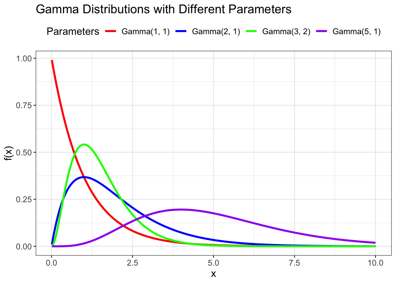
# Gamma distribution with different shape and rate parameters
x <- seq(0.01, 10, .01)
shape_params <- c(1, 2, 3, 5)
rate_params <- c(1, 1, 2, 1)

# Create data for different gamma distributions
gamma_data <- data.frame()
for(i in 1:length(shape_params)) {
  temp_data <- data.frame(
    x = x,
    density = dgamma(x, shape = shape_params[i], rate = rate_params[i]),
    distribution = paste0("Gamma(", shape_params[i], ", ", rate_params[i], ")")
  )
  gamma_data <- rbind(gamma_data, temp_data)
}

# Plot the distributions
ggplot(gamma_data) +
  geom_path(aes(x = x, y = density, color = distribution), linewidth = 1.2) +
  scale_color_manual(values = c("red", "blue", "green", "purple")) +
  labs(x = "x", y = "f(x)",
       title = "Gamma Distributions with Different Parameters",
       color = "Parameters") +
  theme_bw() +
  theme(legend.position = "top", text = element_text(size = 13))

Marginal, Joint, And Conditional Distribution

Moving from One to Multiple Random Variables

• When more than one random variable is present, there are several different types of statistical distributions:

• We will first consider two discrete random variables:

  • x is the outcome of the flip of a penny {\(H_p\), \(T_p\)}

    • \(f(x=H_p) = .5\); \(f(x =T_p) = .5\)

  • z is the outcome of the flip of a dime {\(H_d\), \(T_d\)}

    • \(f(z=H_d) = .5\); \(f(z =T_d) = .5\)

• We will consider the following distributions:

  • Marginal distribution

    • The distribution of one variable only (either \(f(x)\) or \(f(z)\))

  • Joint distribution

    • \(f(x, z)\): the distribution of both variables (both x and z)

  • Conditional distribution

    • The distribution of one variable, conditional on values of the other:

      • \(f(x|z)\): the distribution of x given z

      • \(f(z|x)\): the distribution of z given x

Marginal Distribution

• Marginal distributions are what we have worked with exclusively up to this point: they represent the distribution by itself

  • Continuous univariate distributions

    • Adult heights (Normal)

    • Time between arrivals (Exponential)

    • Device lifetimes (Weibull)

    • Proportions on [0,1] (Beta)

  • Categorical distributions

    • The flip of a penny

    • The flip of a dime

    • The roll of a fair die (1–6)

    • Day of the week (Mon–Sun)

Visualization of marginal and joint distribution

library(ggplot2)

# Marginal categorical distribution: fair die
die <- data.frame(face = factor(1:6), p = rep(1/6, 6))
p1 <- ggplot(die, aes(x = face, y = p)) +
  geom_col(fill = "#5DA5DA") +
  labs(title = "Marginal: Fair Die", x = "Face", y = "Probability") +
  scale_y_continuous(limits = c(0, 0.25)) +
  theme_minimal(base_size = 12)

# Joint categorical distribution: penny × dime (independent, fair)
joint <- expand.grid(penny = c("H", "T"), dime = c("H", "T"))
joint$p <- 0.25
p2 <- ggplot(joint, aes(x = penny, y = dime, fill = p)) +
  geom_tile(color = "white") +
  geom_text(aes(label = scales::percent(p)), color = "black") +
  scale_fill_gradient(low = "#CFE8F3", high = "#2166AC", labels = scales::percent) +
  labs(title = "Joint: Penny × Dime", x = "Penny", y = "Dime", fill = "Probability") +
  theme_minimal(base_size = 12)

p1
p2

Figure 1: marginal (die) distribution

Figure 2: joint (penny × dime) distribution

Joint Distribution

• Joint distributions describe the simultaneous distribution of more than one variable

  • These represent multiple variables collected together

  • Commonly, the joint distribution function is denoted with all random variables separated by commas

  • In our example, \(f(x,z)\) is the joint distribution of the outcome of flipping both a penny and a dime

    • As both are discrete, the joint distribution has four possible values:

      (1) \(f(x = H_p,z=H_d)\) (2) \(f(x = H_p,z=T_d)\) (3) \(f(x = T_p,z=H_d)\) (4) \(f(x = T_p,z=T_d)\)

• Joint distributions are multivariate distributions

• We will use joint distributions to introduce two topics

  • Joint distributions of independent variables

  • Joint distributions – used in maximum likelihood estimation

Joint Distributions of Independent Random Variables

• Random variables are said to be independent if the occurrence of one event makes it neither more nor less probable of another event

  • For joint distributions, this means: \(f(x,z)=f(x)f(z)\)

• In our example, flipping a penny and flipping a dime are independent – so we can complete the following table of their joint distribution:

  	z = \(H_d\)	z = \(T_d\)	Marginal (Penny)
  \(x = H_p\)	\(\color{tomato}{f(x=H_p, z=H_d)}\)	\(\color{tomato}{f(x=H_p, z=T_d)}\)	\(\color{turquoise}{f(z=H_p)}\)
  \(x = T_p\)	\(\color{tomato}{f(x= T_p, z=H_d)}\)	\(\color{tomato}{f(x=T_p, z=T_d)}\)	\(\color{turquoise}{f(z=T_d)}\)
  Marginal (Dime)	\(\color{turquoise}{f(z=H_d)}\)	\(\color{turquoise}{f(z=T_d)}\)

Joint Distributions of Independent Random Variables

• Because the coin flips are independent, this becomes:

	z = \(H_d\)	z = \(T_d\)	Marginal (Penny)
\(x = H_p\)	\(\color{tomato}{f(x=H_p)f( z=H_d)}\)	\(\color{tomato}{f(x=H_p)f( z=T_d)}\)	\(\color{turquoise}{f(z=H_p)}\)
\(x = T_p\)	\(\color{tomato}{f(x= T_p)f( z=H_d)}\)	\(\color{tomato}{f(x=T_p)f( z=T_d)}\)	\(\color{turquoise}{f(z=T_d)}\)
Marginal (Dime)	\(\color{turquoise}{f(z=H_d)}\)	\(\color{turquoise}{f(z=T_d)}\)

• Then, with numbers:

	z = \(H_d\)	z = \(T_d\)	Marginal (Penny)
\(x = H_p\)	\(\color{tomato}{.25}\)	\(\color{tomato}{.25}\)	\(\color{turquoise}{.5}\)
\(x = T_p\)	\(\color{tomato}{.25}\)	\(\color{tomato}{.25}\)	\(\color{turquoise}{.5}\)
Marginal (Dime)	\(\color{turquoise}{.5}\)	\(\color{turquoise}{.5}\)

Marginalizing Across a Joint Distribution

• If you had a joint distribution, \(\color{orchid}{f(x, z)}\), but wanted the marginal distribution of either variable (\(f(x)\) or \(f(z)\)) you would have to marginalize across one dimension of the joint distribution.

• For categorical random variables, marginalizing means summing across every value of z

\[ f(x) = \sum_zf(x, z) \]

• For example, \(f(x = H_p) = f(x = H_p, z=H_d) +f(x = H_p, z=T_d)=.5\)

• For continuous random variables, marginalizing means integrating across z

  • The integral:

    \[ f(x) = \int_zf(x,z)dz \]

Conditional Distribution

• For two random variables x and z, a conditional distribution is written as: \(f(z|x)\)

  • The distribution of z given x

• The conditional distribution equals the joint distribution divided by the marginal distribution of the conditioning variable

  \[ f(z|x) = \frac{f(z,x)}{f(x)} \]

• Conditional distributions are found everywhere in statistics

  • The general linear model uses the conditional distribution of the variable

    \[ Y \sim N(\beta_0+\beta_1X, \sigma^2_e) \]

Example: Conditional Distribution

• For two discrete random variables with {0, 1} values, the conditional distribution can be shown in a contingency table:

	z = \(H_d\)	z = \(T_d\)	Marginal (Penny)
\(x = H_p\)	\(\color{tomato}{.25}\)	\(\color{tomato}{.25}\)	\(\color{turquoise}{.5}\)
\(x = T_p\)	\(\color{tomato}{.25}\)	\(\color{tomato}{.25}\)	\(\color{turquoise}{.5}\)
Marginal (Dime)	\(\color{turquoise}{.5}\)	\(\color{turquoise}{.5}\)

Conditional: \(f(z | x= H_p)\):

\(f(z=H_d|x =H_p) = \frac{f(z=H_d, x=H_p)}{f(x = H_p)} = \frac{.25}{.5}=.5\)

\(f(z = T_d | x = H_p)= \frac{f(z=T_d, x=H_p)}{f(x=H_p)} = \frac{.25}{.5} = .5\)

Exercise: calculate conditional probabilities

Using the same penny (x) and dime (z) setup, suppose the joint distribution is slightly modified as follows:

	z = \(H_d\)	z = \(T_d\)
\(x = H_p\)	0.30	0.20
\(x = T_p\)	0.20	0.30

• Compute the marginal probabilities: \(P(x=H_p)\), \(P(x=T_p)\), \(P(z=H_d)\), \(P(z=T_d)\).
• Compute the conditional probabilities: \(P(z=H_d\mid x=H_p)\) and \(P(x=T_p\mid z=T_d)\).
• Briefly show your work (fractions from the table entries).

Answer (click to expand)

Marginals:

• \(P(x=H_p) = 0.30 + 0.20 = 0.50\)
• \(P(x=T_p) = 0.20 + 0.30 = 0.50\)
• \(P(z=H_d) = 0.30 + 0.20 = 0.50\)
• \(P(z=T_d) = 0.20 + 0.30 = 0.50\)

Conditionals:

• \(P(z=H_d\mid x=H_p) = \dfrac{0.30}{0.50} = 0.60\)
• \(P(x=T_p\mid z=T_d) = \dfrac{0.30}{0.50} = 0.60\)

Expected Values and The Algebra of Expectation

Expected Values

• Expected values are statistics calculated over the sample space of a random variable: they are essentially weighted averages:

  set.seed(1234)
  x = rnorm(100, mean = 0, sd = 1)
  w = dnorm(x, mean = 0, sd = 1)
  mean(w * x)

  [1] -0.05567835

• Where \(w\) denotes the density function of x: \(f(x)\)

• The weights used in computing this average correspond to the probabilities (for discrete random variables) or the densities (for continuous random variables)

Note

The expected value is represented by \(E(x)\)

The actual statistic being weighted by the PDF is placed in the parentheses where x appears

• Expected values allow us to understand what a statistical model implies about data, for instance:

  • How a GLM specifies the (conditional) mean and variance of a DV

Expected Value Calculation

• For discrete random variables, the expected value is found by:

  \[ E(x) = \sum{x \times P(X=x)} \]

• For example, the expected value of a roll of a die is:

  \[ E(x) = (1)\frac16+ (2)\frac16+(3)\frac16+(4)\frac16+(5)\frac16+6\frac16 \]

• For continuous random variables, the expected value is found by

  \[ E(x) = \int_x xf(x)dx \]

• We won’t be calculating theoretical expected values using calculus… we use them only to understand what our models imply about the data

Variance and Covariance… As Expected Values

• A distribution’s theoretical variance can also be written as an expected value:

  \[ V(x) = E(x-E(x))^2 = E(x -\mu_x)^2 \]

  • This formula helps us understand predictions made by GLMs and how that corresponds to statistical parameters we interpret

• For a roll of a die, the theoretical variance is:

  \[ V(x) = E(x - 3.5)^2 = \frac16(1-3.5)^2 + \frac16(2-3.5)^2 + \frac16(3-3.5)^2 + \frac16(4-3.5)^2 + \frac16(5-3.5)^2 + \frac16(6-3.5)^2 = 2.92 \]

• Likewise, for a pair of random variable x and z, the covariance can be found from their joint distributions:

  \[ \text{Cov}(x,z)=E(xz)-E(x)E(z) = E(xz)-\mu_x\mu_z \]

set.seed(1234)
N = 100
x = rnorm(N, 2, 1)
z = rnorm(N, 3, 1)
xz = x*z
(Cov_xz = mean(xz)-mean(x)*mean(z)) / ((N-1)/N) # unbiased covariance
cov(x, z)

[1] -0.02631528
[1] -0.02631528

Linear Combination of Random Variables

Linear Combinations of Random Variables

• A linear combination is an expression constructed from a set of terms by multiplying each term by a constant and then adding the results \[ x = c + a_1z_1+a_2z_2+a_3z_3 +\cdots+a_nz_n \]

• More generally, linear combinations of random variables have specific implications for the mean, variance, and possibly covariance of the new random variable

• As such, there are predictable ways in which the means, variances, and covariances change

Algebra of Expectations

• Sums of Constants

\[ E(x+c) = E(x)+c \\ \text{Var}(x+c) = \text{Var}(x) \\ \text{Cov}(x+c, z) = \text{Cov}(x, z) \]

Example

Imagine for weight variable, each individual increases 3 lbs:

set.seed(1234)
library(ESRM64503)
x = dataSexHeightWeight$weightLB
c_ = 3
z = dataSexHeightWeight$heightIN
mean(x + c_); mean(x)+c_

[1] 186.4

[1] 186.4

var(x + c_); var(x)

[1] 3179.095

[1] 3179.095

cov(x, z); cov(x+c_, z) # decimal place issue, near() accepts two values' diff less than .00001

[1] 334.8316

[1] 334.8316

• Products of Constants:

\[ E(cx) = cE(x) \\ \text{Var}(cx) = c^2\text{Var}(x) \\ \text{Cov}(cx, dz) = c*d*\text{Cov}(x, z) \] Imagine you wanted to convert weight from pounds to kilograms (where 1 pound = 0.453 kg) and convert height from inches to cm (where 1 inch = 2.54 cm)

c_ = .453
mean(x*c_); mean(x)*c_

[1] 83.0802

[1] 83.0802

var(x*c_); var(x)*c_^2

[1] 652.3789

[1] 652.3789

d_ = 2.54
cov(c_*x, d_*z);c_*d_*cov(x, z)

[1] 385.2639

[1] 385.2639

• Sums of Multiple Random Variables:

\[ E(cx+dz) = cE(x) + dE(z) \\ \text{Var}(cx+dz) = c^2\text{Var}(x) + d^2\text{Var}(z) + 2c*d*\text{Cov}(x,z)\\ \]

mean(x*c_+z*d_); mean(x)*c_+mean(z)*d_

[1] 255.5462

[1] 255.5462

var(x*c_+z*d_); c_^2*var(x) + d_^2*var(z) + 2*c_*d_*cov(x, z)

[1] 1780.054

[1] 1780.054

Where We Use This Algebra

• Recall how we calculated the standard error of the conditional main effect using the simple main effect and interaction effect

\[ \mathbf{Test = 82.20 + 2.16*Senior + 7.76*New - 3.04*Senior*New} \]

• The conditional main effect of Senior when New equals 1 is (2.16 - 3.04) = -0.88

  • We know that \(\text{Var}(\beta_{\text{Senior}})\) is 0.575, \(\text{Var}(\beta_{\text{Senior*New}})\) is 1.151, and \(\text{Cov}(\beta_{\text{Senior}}, \beta_{\text{Senior*New}})\) is -0.575.

model1 <- lm(Test ~ Senior + New + Senior * New, data = dataTestExperiment)
vcov(model1)

            (Intercept)     Senior        New Senior:New
(Intercept)   0.2877333 -0.2877333 -0.2877333  0.2877333
Senior       -0.2877333  0.5754667  0.2877333 -0.5754667
New          -0.2877333  0.2877333  0.5754667 -0.5754667
Senior:New    0.2877333 -0.5754667 -0.5754667  1.1509333

Then,

\[ \mathbf{Var(\beta_{Senior}+\beta_{Senior*New}) = Var(\beta_{Senior}) + Var(\beta_{Senior*New}) + 2Cov(\beta_{Senior},\beta_{Senior*New}) \\ = 0.575 + 1.151 - 2* 0.575 = 0.576} \] Thus, \(SE(\beta_{Senior}+\beta_{Senior*New})=0.759\)

Combining the GLM with Expectations

• Using the algebra of expectations for predicting Y from X and Z:

\[ \hat{Y}_p=E(Y_p)=E(\beta_0+\beta_1X_p+\beta_2Z_p+\beta_3X_pZ_p+e_p) \\ = \beta_0+\beta_1X_p+\beta_2Z_p+\beta_3X_pZ_p+E(e_p) \\ = \beta_0+\beta_1X_p+\beta_2Z_p+\beta_3X_pZ_p \]

• The variance of \(f(Y_p|X_p, Z_p)\):

\[ V(\hat{Y_P}|X_p, Z_p)=V(\beta_0+\beta_1X_p+\beta_2Z_p+\beta_3X_pZ_p+e_p)\\ = V(\hat{Y}_p + e_p)=\sigma_e^2 \]

Understanding These Concepts in the Context of Data

• Recall from the regression analysis of the height/weight data that the final model we decided to interpret was Model 5

\[ W_p = \beta_0+\beta_1 (H_p-\bar{H}) +\beta_2F_p+\beta_3 (H_p-\bar{H}) F_p + e_p \]

where \(e_p \sim N(0, \sigma_e^2)\)

dat <- dataSexHeightWeight
dat$heightIN_MC <- dat$heightIN - mean(dat$heightIN)
dat$female <- dat$sex == 'F'
mod5 <- lm(weightLB ~ heightIN_MC + female + female*heightIN_MC, data = dat)
summary(mod5)

Call:
lm(formula = weightLB ~ heightIN_MC + female + female * heightIN_MC, 
    data = dat)

Residuals:
    Min      1Q  Median      3Q     Max 
-3.8312 -1.7797  0.4958  1.3575  3.3585 

Coefficients:
                       Estimate Std. Error t value Pr(>|t|)    
(Intercept)            222.1842     0.8381  265.11  < 2e-16 ***
heightIN_MC              3.1897     0.1114   28.65 3.55e-15 ***
femaleTRUE             -82.2719     1.2111  -67.93  < 2e-16 ***
heightIN_MC:femaleTRUE  -1.0939     0.1678   -6.52 7.07e-06 ***
---
Signif. codes:  0 '***' 0.001 '**' 0.01 '*' 0.05 '.' 0.1 ' ' 1

Residual standard error: 2.175 on 16 degrees of freedom
Multiple R-squared:  0.9987,    Adjusted R-squared:  0.9985 
F-statistic:  4250 on 3 and 16 DF,  p-value: < 2.2e-16

Picturing the GLM with Distributions

• The distributional assumptions of the GLM explain why we do not need to worry about whether our dependent variable is normally distributed

• Our dependent variable should be conditionally normal

• We can check this assumption by examining the residuals: \(e_p \sim N(0, \sigma^2_e)\)

Assessing Distributional Assumptions Graphically

plot(mod5)

Hypothesis Tests for Normality

If a given test is significant, it indicates that your data do not come from a normal distribution

In practice, tests will often provide conflicting information. The best way to evaluate normality is to consider both plots and tests together (approximate normality is usually sufficient)

shapiro.test(mod5$residuals)

    Shapiro-Wilk normality test

data:  mod5$residuals
W = 0.95055, p-value = 0.3756

Wrapping Up

• Today was an introduction to mathematical statistics as a way to understand the implications statistical models make about data

• Although many of these topics do not seem directly relevant, they help provide insights that untrained analysts may not easily attain