flowchart RL
    A("Model:
      Substantive Theory") --> |Hypothesized Causal Process|B("Observed Outcomes
                                                                 (any format)")
Lecture 06: Generalized Linear Models (Binary Outcome) and Matrix Algebra
Generalized Linear Models
Jihong Zhang*, Ph.D
Educational Statistics and Research Methods (ESRM) Program*
University of Arkansas
2024-09-24
Today’s Class
- Introduction to Generalized Linear Models
- Expanding your linear models knowledge to models for outcomes that are not conditionally normally distributed
- An example of generalized models for binary data using logistic regression
- Matrix Algebra
An Introduction to Generalized Linear Models
Categories of Multivariate Models
Statistical models can be broadly organized as:
- General (normal outcome) vs. Generalized (not normal outcome)
- One dimension of sampling (one variance term per outcome) vs. multiple dimensions of sampling (multiple variance terms)
- Fixed effects only vs. Mixed effects (fixed and random effects = multilevel)
All models have fixed effects, and then:
- General Linear Models (GLM): conditionally normal distribution of data, fixed effects and no random effects
- General Linear Mixed Models (GLMM): conditionally normal distribution for data, fixed and random effects
- Generalized Linear Models: any conditional distribution for data, fixed effects through link functions, no random effects
- Generalized Linear Mixed Models: any conditional distribution for data, fixed effects through link functions, fixed and random effects
“Linear” means the fixed effects predict the link-transformed DV in a linear combination of the form:
\[ g^{-1}(\beta_0 +\beta_1X_1+ \beta_2X_2 + \cdots) \]
Unpacking the Big Picture
Substantive theory: the guiding framework for your study
Hypothetical causal process: what the statistical model is testing (attempting to falsify) when estimated
Observed outcomes: what you collect and evaluate based on your theory
Outcomes can take many forms:
Continuous variables (e.g., time, blood pressure, height)
Categorical variables (e.g., Likert-type response, ordered categories, nominal categories)
Combinations of continuous and categorical (e.g., either 0 or some other continuous number)
The Goal of Generalized Models
Generalized models connect a substantive theory to the sample space (the range of possible values) of the observed outcomes
- Sample space = type/range/outcomes that are possible
The core idea is that a statistical model will not approximate the outcome well if its assumed distribution is a poor fit for the outcome’s sample space.
- If model does not fit the outcome, the findings cannot be trusted
The key to making all of this work is the use of differing statistical distributions for the outcome
Generalized models allow for different distributions for outcomes
- The mean of the distribution is still modeled by the model for the means (the fixed effects)
- The variance of the distribution may or may not be modeled (some distributions don’t have variance terms)
What kind of outcome? Generalized vs. General
Generalized Linear Models are an extension of General Linear Models for outcomes with non-normal residuals. They predict a transformed Y (via a link function) instead of Y on its original scale
Many kinds of non-normally distributed outcomes have some kind of generalized linear model to go with them:
- Binary (dichotomous)
- Unordered categorical (nominal)
- Ordered categorical (ordinal) These two are often called “multinomial” inconsistently
- Counts (discrete, positive values)
- Censored (piled up and cut off at one end – left or right)
- Zero-inflated (pile of 0’s, then some distribution after)
- Continuous but skewed data (pile on one end, long tail)
Common distributions and canonical link functions (from Wikipedia)
| Distribution | Support of distribution | Typical uses | Link name | Link function \({\displaystyle \mathbf {X} {\boldsymbol {\beta }}=g(\mu )\,\!}\) |
Mean function |
|---|---|---|---|---|---|
| Normal | real: \({\displaystyle (-\infty ,+\infty )}\) |
Linear-response data | Identity | \({\displaystyle \mathbf {X} {\boldsymbol {\beta }}=\mu \,\!}\) |
\({\displaystyle \mu =\mathbf {X} {\boldsymbol {\beta }}\,\!}\) |
| Exponential | real: \({\displaystyle (0,+\infty )}\) |
Exponential-response data, scale parameters | Negative inverse | \({\displaystyle \mathbf {X} {\boldsymbol {\beta }}=-\mu ^{-1}\,\!}\) |
\({\displaystyle \mu =-(\mathbf {X} {\boldsymbol {\beta }})^{-1}\,\!}\) |
| Gamma | |||||
| Inverse Gaussian |
real: \({\displaystyle (0,+\infty )}\) |
Inverse squared |
\({\displaystyle \mathbf {X} {\boldsymbol {\beta }}=\mu ^{-2}\,\!}\) |
\({\displaystyle \mu =(\mathbf {X} {\boldsymbol {\beta }})^{-1/2}\,\!}\) |
|
| Poisson | integer: \({\displaystyle 0,1,2,\ldots }\) |
count of occurrences in fixed amount of time/space | Log | \({\displaystyle \mathbf {X} {\boldsymbol {\beta }}=\ln(\mu )\,\!}\) |
\({\displaystyle \mu =\exp(\mathbf {X} {\boldsymbol {\beta }})\,\!}\) |
| Bernoulli | integer: \({\displaystyle \{0,1\}}\) |
outcome of single yes/no occurrence | Logit | \({\displaystyle \mathbf {X} {\boldsymbol {\beta }}=\ln \left({\frac {\mu }{1-\mu }}\right)\,\!}\) |
\({\displaystyle \mu ={\frac {\exp(\mathbf {X} {\boldsymbol {\beta }})}{1+\exp(\mathbf {X} {\boldsymbol {\beta }})}}={\frac {1}{1+\exp(-\mathbf {X} {\boldsymbol {\beta }})}}\,\!}\) |
| Binomial | integer: \({\displaystyle 0,1,\ldots ,N}\) |
count of # of "yes" occurrences out of N yes/no occurrences | \({\displaystyle \mathbf {X} {\boldsymbol {\beta }}=\ln \left({\frac {\mu }{n-\mu }}\right)\,\!}\) |
||
| Categorical | integer: \({\displaystyle [0,K)}\) |
outcome of single K-way occurrence | \({\displaystyle \mathbf {X} {\boldsymbol {\beta }}=\ln \left({\frac {\mu }{1-\mu }}\right)\,\!}\) |
||
K-vector of integer: \({\displaystyle [0,1]}\)![{\displaystyle [0,1]}](https://wikimedia.org/api/rest_v1/media/math/render/svg/738f7d23bb2d9642bab520020873cccbef49768d) , where exactly one element in the vector has the value 1 , where exactly one element in the vector has the value 1 |
|||||
| Multinomial | K-vector of integer: \({\displaystyle [0,N]}\)![{\displaystyle [0,N]}](https://wikimedia.org/api/rest_v1/media/math/render/svg/703d57dca548a7f9d927247c2a27b67666aebdd5) |
count of occurrences of different types (1, ..., K) out of N total K-way occurrences |
Three Parts of a Generalized Linear Model
Link Function \(g(\cdot)\) (main difference from GLM):
How a non-normal outcome gets transformed into something we can predict that is more continuous (unbounded)
For outcomes that are already normal, general linear models are just a special case with an “identity” link function (Y * 1)
Model for the Means (“Structural Model”):
How predictors are linearly related to the link-transformed outcome (or non-linearly related to the outcome on its original scale)
New link-transformed \(Y_p = \color{royalblue}{g^{-1}} (\color{tomato}{\mathbf{\beta_0}} + \color{tomato}{\mathbf{\beta_1}}X_p + \color{tomato}{\mathbf{\beta_2}} Z_p + \color{tomato}{\mathbf{\beta_3}} X_pZ_p)\)
Model for the Variance (“Sampling/Stochastic Model”):
- If the errors aren’t normally distributed, then what are they?
- Family of alternative distributions at our disposal that map onto what the distribution of errors could possibly look like
- In logistic regression, you often hear sayings like “no error term exists” or “the error term has a binomial distribution” (more accurately, the variance is determined by the mean, following a binomial distribution).
Link Functions: How Generalized Models Work
Generalized models work by providing a mapping of the theoretical portion of the model (the right hand side of the equation) to the sample space of the outcome (the left hand side of the equation)
- The mapping is performed by a link function
The link function is a non-linear function that takes the linear model predictors, random/latent terms, and constants and puts them onto the space of the outcome observed variables
Link functions are typically expressed for the mean of the outcome variable (we will only focus on that)
- In generalized models, the error variance is often a function of the mean, so no additive information exists if estimating the error term
Link Functions in Practice
- The link function expresses the conditional value of the mean of the outcome
\[ E(Y_p) = \hat{Y}_p = \mu_y \]
where \(E(\cdot)\) stands for expectation.
… through a non-linear link function \(g(\hat Y_p)\) when used on conditional mean of outcome
or its inverse link function \(g^{-1}(\mathbf{\beta X})\) when used on linear combination of predictors
The general form is:
\[ E(Y_p) =\hat{Y}_p = \mu_y =\color{royalblue}{g^{-1}}(\color{tomato}{\beta_0+\beta_1X_p+\beta_2Z_p+\beta_3X_pZ_p}) \]
The red part is the linear combination of predictors and their effects.
Why normal GLM is one type of Generalized Linear Model
- Our familiar general linear model is actually a member of the generalized model family (it is subsumed)
- The link function is called the identity, the linear predictor is unchanged
- The normal distribution has two parameters, a mean \(\mu\) and a variance \(\sigma^2\)
- Unlike most distributions, the normal distribution parameters are directly modeled by the GLM
- In conditionally normal GLMs, the inverse link function is called the identity function:
\[ g^{-1}(\cdot) = \boldsymbol{I}(\cdot) = 1 * (\color{yellowgreen}{\text{linear combination of predictors}}) \]
The identity function does not alter the predicted values – they can be any real number
This matches the sample space of the normal distribution – the mean can be any real number
- The expected value of an outcome from the GLM is:
\[ \begin{align} \mathbb{E}(Y_p) =\hat{Y}_p = \mu_y &=\color{royalblue}{\boldsymbol{I}}(\color{yellowgreen}{\beta_0+\beta_1X_p+\beta_2Z_p+\beta_3X_pZ_p}) \\ &= \beta_0+\beta_1X_p+\beta_2Z_p+\beta_3X_pZ_p \end{align} \]
About the Variance of GLM
The other parameter of the normal distribution described the variance of an outcome – called the error (residual) variance
We found that the model for the variance for the GLM was:
\[ \begin{align} Var(Y_p) &= Var(\beta_0+\beta_1X_p+\beta_2Z_p+\beta_3X_pZ_p + \color{tomato}{e}_p ) \\ &= Var(e_p) \\ &= \sigma^2_e \end{align} \]
- Similarly, this term directly relates to the variance of the outcome in the normal distribution
- We will quickly see distributions from other families (i.e., logistic ) where this doesn’t happen
- Error terms are independent of predictors
Generalized Linear Models For Binary Data
Today’s Data Example
- To help demonstrate generalized models for binary data, we borrow from an example listed on the UCLA ATS website.
- The data is available after updating the
ESRM64503package - The data come from a survey of 400 college juniors looking at factors that influence the decision to apply to graduate school:
- Y (outcome): a student’s rated likelihood of applying to grad school (0 = unlikely; 1 = somewhat likely; 2 = very likely)
- We will first look at Y for two categories (0 = unlikely; 1 = somewhat or very likely) – we merged the ‘somewhat likely’ and ‘very likely’ categories for this illustration.
- In practice, you would typically use a model designed for three or more ordered categories (like an ordinal logistic regression).
- ParentEd: indicator (0/1) if one or more parent has graduate degree
- Public: indicator (0/1) if student attends a public university
- GPA: grade point average on 4 point scale (4.0 = perfect)
- Y (outcome): a student’s rated likelihood of applying to grad school (0 = unlikely; 1 = somewhat likely; 2 = very likely)
Descriptive Statistics for Data
Code
library(ESRM64503)
library(tidyverse)
library(kableExtra)
Desp_GPA <- dataLogit |>
  summarise(
    Variable = "GPA",
    N = n(),
    Mean = mean(GPA),
    `Std Dev` = sd(GPA),
    Minimum = min(GPA),
    Maximum = max(GPA)
  )

Desp_Apply <- dataLogit |>
  group_by(APPLY) |>
  summarise(
    Frequency = n(),
    Percent = n() / nrow(dataLogit) * 100
  ) |>
  ungroup() |>
  mutate(
    `Cumulative Frequency` = cumsum(Frequency),
    `Cumulative Percent` = cumsum(Percent)
  )

Desp_LLApply <- dataLogit |>
  group_by(LLAPPLY) |>
  summarise(
    Frequency = n(),
    Percent = n() / nrow(dataLogit) * 100
  ) |>
  ungroup() |>
  mutate(
    `Cumulative Frequency` = cumsum(Frequency),
    `Cumulative Percent` = cumsum(Percent)
  )


Desp_PARED <- dataLogit |>
  group_by(PARED) |>
  summarise(
    Frequency = n(),
    Percent = n() / nrow(dataLogit) * 100
  ) |>
  ungroup() |>
  mutate(
    `Cumulative Frequency` = cumsum(Frequency),
    `Cumulative Percent` = cumsum(Percent)
  )

Desp_PUBLIC <- dataLogit |>
  group_by(PUBLIC) |>
  summarise(
    Frequency = n(),
    Percent = n() / nrow(dataLogit) * 100
  ) |>
  ungroup() |>
  mutate(
    `Cumulative Frequency` = cumsum(Frequency),
    `Cumulative Percent` = cumsum(Percent)
)| APPLY | Frequency | Percent | Cumulative Frequency | Cumulative Percent |
|---|---|---|---|---|
| 0 | 220 | 55 | 220 | 55 |
| 1 | 140 | 35 | 360 | 90 |
| 2 | 40 | 10 | 400 | 100 |
| LLAPPLY | Frequency | Percent | Cumulative Frequency | Cumulative Percent |
|---|---|---|---|---|
| 0 | 220 | 55 | 220 | 55 |
| 1 | 180 | 45 | 400 | 100 |
| Variable | N | Mean | Std Dev | Minimum | Maximum |
|---|---|---|---|---|---|
| GPA | 400 | 2.998925 | 0.3979409 | 1.9 | 4 |
| PARED | Frequency | Percent | Cumulative Frequency | Cumulative Percent |
|---|---|---|---|---|
| 0 | 337 | 84.25 | 337 | 84.25 |
| 1 | 63 | 15.75 | 400 | 100.00 |
| PUBLIC | Frequency | Percent | Cumulative Frequency | Cumulative Percent |
|---|---|---|---|---|
| 0 | 343 | 85.75 | 343 | 85.75 |
| 1 | 57 | 14.25 | 400 | 100.00 |
What If We Used a Normal GLM for Binary Outcomes?
- If \(Y_p\) is a binary (0 or 1) outcome
- Expected mean is proportion of people who have a 1 (or “p”, the probability of Y_p = 1 in the sample)
- The probability of having a 1 is what we’re trying to predict for each person, given the values of his/her predictors
- General linear model: \(Y_p = I(\beta_0 + \beta_1x_p + \beta_2z_p + e_p)\)
- \(\color{tomato}{\beta}_0\) = expected probability when all predictors are 0
- \(\color{tomato}{\beta}_s\) = expected change in probability for a one-unit change in the predictor
- \(\color{royalblue}{e}_p\) = difference between observed and predicted values
- Generalized Linear Model becomes \(Y_p = \color{tomato}{(\text{predicted probability of outcome equal to 1})} + e_p\)
A General Linear Model of Predicting Binary Outcomes?
But if \(Y_p\) is binary and link function is identity link, then \(e_p\) can only be 2 things:
\(e_p\) = \(Y_p - \hat{Y}_p\)
If \(Y_p = 0\) then \(e_p\) = (0 - predicted probability)
If \(Y_p = 1\) then \(e_p\) = (1 - predicted probability)
The mean of errors would still be 0 … by definition
However, the variance of the errors cannot be constant across levels of X, as is assumed in general linear models
The mean and variance of a binary outcome are dependent!
As shown shortly, mean = p and variance = p * (1 - p), so they are tied together
This means that because the conditional mean of Y (p, the predicted probability Y = 1) is dependent on X, then so is the error variance, violating the assumption of homoscedasticity.
A General Linear Model With Binary Outcomes?
How can we have a linear relationship between X & Y?
Probability of a 1 is bounded between 0 and 1, but predicted probabilities from a linear model aren’t bounded
- Impossible values
The linear relationship needs to ‘shut off’ at the 0 and 1 boundaries, which requires a non-linear function.
Predicted Regression Line of GLM
Code
library(ggplot2)
ggplot(dataLogit) +
  aes(x = GPA, y = LLAPPLY) +
  geom_hline(aes( yintercept = 1)) +
  geom_hline(aes( yintercept = 0)) +
  geom_point(color = "tomato", alpha = .8) +
  geom_smooth(method = "lm", se = FALSE, fullrange = TRUE, linewidth = 1.3) +
  scale_x_continuous(limits = c(0, 8), breaks = 0:8) +
  scale_y_continuous(limits = c(-0.4, 1.4), breaks = seq(-0.4, 1.4, .1)) +
  labs(y = "Predicted Probability of Y") +
  theme_classic() +
  theme(text = element_text(size = 20))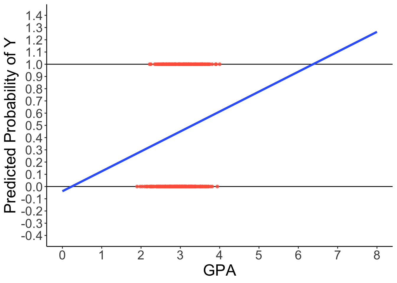
Predicted Regression Line of Logistic Regression
Code
ggplot(dataLogit) +
  aes(x = GPA, y = LLAPPLY) +
  geom_hline(aes( yintercept = 1)) +
  geom_hline(aes( yintercept = 0)) +
  geom_point(color = "tomato", alpha = .8) +
  geom_smooth(method = "glm", se = FALSE, fullrange = TRUE,
              method.args = list(family = binomial(link = "logit")), color = "yellowgreen", linewidth = 1.5) +
  scale_x_continuous(limits = c(0, 8), breaks = 0:8) +
  scale_y_continuous(limits = c(-0.4, 1.4), breaks = seq(-0.4, 1.4, .1)) +
  labs(y = "Predicted Probability of Y") +
  theme_classic() +
  theme(text = element_text(size = 20))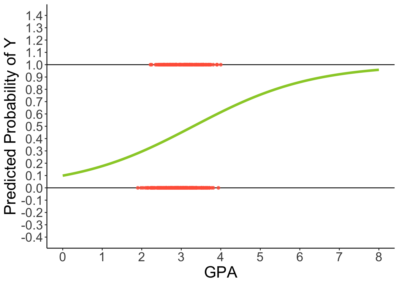
3 Problems with GLM predicting binary outcomes
Assumption Violation problem: GLM for continuous, conditionally normal outcome = residuals can’t be normally distributed
Restricted Range problem (e.g., 0 to 1 for outcomes)
Predictors should not be linearly related to observed outcome
- Effects of predictors need to be ‘shut off’ at some point to keep predicted values of binary outcome within range
Decision-Making Problem: A GLM predicts a continuous value, but the research question is often binary (e.g., ‘will a student apply?’). It’s unclear how to make a decision from a continuous prediction that can be outside the 0-1 range.
- In contrast, a generalized linear model provides a probability (e.g., ‘a student has a 50% probability of applying’), which directly answers the question.
The Binary Outcome: Bernoulli Distribution
Bernoulli distribution has following properties
Notation: \(Y_p \sim B(\boldsymbol{p}_p)\) (where p is the conditional probability of a 1 for person p)
Sample Space: \(Y_p \in \{0, 1\}\) (\(Y_p\) can either be a 0 or a 1)
Probability Density Function (PDF):
- \[ f(Y_p) = (\mathbf{p}_p)^{Y_p}(1-\mathbf{p}_p)^{1-Y_p} \]
Expected value (mean) of Y: \(E(y_p) = \mu_{Y_p}=\boldsymbol{p}_p\)
Variance of Y: \(Var(Y_p) = \sigma^2_{Y_p} = \boldsymbol{p}_p ( 1- \boldsymbol{p}_p )\)
Note
\(\boldsymbol{p}_p\) is the only parameter – so we only need to provide a link function for it …
Generalized Models for Binary Outcomes
Rather than modeling the probability of a 1 directly, we need to transform it into a more continuous variable with a link function, for example:
We could transform probability into an odds ratio
Odds ratio (OR): \(\frac{p}{1-p} = \frac{Pr(Y = 1)}{Pr(Y = 0)}\)
For example, if \(p = .7\), then OR(1) = 2.33; OR(0) = .429
Odds scale is way skewed, asymmetric, and ranges from 0 to \(+\infty\)
- This is not a helpful property
Take natural log of odds ratio \(\rightarrow\) called “logit” link
\(\text{logit}(p) = \log(\frac{p}{1-p})\)
For example, \(\text{logit}(.7) = .847\) and \(\text{logit}(.3) = -.847\)
- Logit scale is now symmetric at \(p = .5\)
The logit link is one of many used for the Bernoulli distribution
- Names of others: Probit, Log-Log, Complementary Log-Log
From Logit Transformation to Logistic Regression
The link function for a logit is defined by:
\[ g(\mathbb{E}(Y)) = \log(\frac{P(Y=1)}{1-P(Y=1)}) = \mathbf{\beta} X^T \tag{1}\]
where \(g\) is called the link function, \(\mathbb{E}(Y)\) is the expectation of Y, \(\beta X^T\) is the linear combination of weights and predictors.
A logit can be translated back to a probability with some algebra:
\[ P(Y=1) = \frac{\exp(\beta X^T)}{1+\exp(\beta X^T)} = \frac{\exp(\beta_0 + \beta_1 X + \beta_2Z + \beta_3XZ)}{1+\exp(\beta_0 + \beta_1 X + \beta_2Z + \beta_3XZ)} \\ = (1+\exp(-1*(\beta_0 + \beta_1 X + \beta_2Z + \beta_3XZ)))^{-1} \tag{2}\]
From Equation 1 and Equation 2, we can know that \(g(\mathbb{E}(Y))\) has a range of [-\(\infty\), +\(\infty\)], P(Y = 1) has a range of [0, 1].
Interpretation of Coefficients
[1] 0.1184699[1] 0.1343912Intercept \(\beta_0\):
Logit: We can say the predicted logit value of Y = 1 for an individual when all predictors are zero; i.e., the average logit is -2.007
Probability: Alternatively, we can say the expected value of probability of Y = 1 is \(\frac{\exp(\beta_0)}{1+\exp(\beta_0)}\) when all predictors are zero; i.e., the average probability of applying to grad school is 0.118 (11.8%)
Odds: Alternatively, the expected odds of Y = 1 is \(\exp(\text{Logit})\) when all predictors are zero. The average odds of applying to grad school is exp(-2.007) = 0.134.
Slope \(\beta_1\):
Logit: We can say the predicted increase of logit value of Y = 1 with one-unit increase of X;
Probability: We can say the expected increase of probability of Y = 1 is \(\frac{\exp(\beta_0+\beta_1)}{1+\exp(\beta_0+\beta_1)}-\frac{\exp(\beta_0)}{1+\exp(\beta_0)}\) with one-unit increase of X; Note that the increase (\(\Delta(\beta_0, \beta_1)\)) is non-linear and dynamic given varied value of X.
Odds Ratio: For a one-unit increase in X, the odds of Y=1 are multiplied by a factor of \(\exp(\beta_1)\). This factor is the odds ratio (OR). (Hint: The new odds are \(\exp(\beta_0+\beta_1) = \exp(\beta_0)\exp(\beta_1)\), which is \(\exp(\beta_1)\) times the old odds of \(\exp(\beta_0)\))
Example: Fitting The Models
Model 0: The empty model for logistic regression with binary variable (applying for grad school) as the outcome
Model 1: The logistic regression model including centered GPA and binary predictors (Parent has graduate degree, Student Attends Public University)
Model 0: The empty model
The statistical form of empty model:
\[ P(Y_p =1) = \frac{\exp(\beta_0)}{1+\exp(\beta_0)} \]
or
\[ \text{logit}(P(Y_p = 1)) = \beta_0 \]
Takehome Note
Many generalized linear models don’t explicitly show an error term. This is because the variance is a function of the mean (e.g., for a binary outcome, variance = p(1-p)).
For the logit function, \(e_p\) has a logistic distribution with a zero mean and a variance as \(\pi^2\)/3 = 3.29.
- Use
ordinalpackage andclm()function, we can model categorical dependent variables.
- 1
-
The dependent variable must be stored as a
factor - 2
-
the
formulaanddataarguments are identical tolm; Thecontrol =argument is only used here to show iteration history of the ML algorithm
iter:  step factor:     Value:     max|grad|:   Parameters:
   0:  1.000000e+00:    277.259:   2.000e+01:   0
nll reduction:  2.00332e+00
   1:  1.000000e+00:    275.256:   6.640e-02:   0.2
nll reduction:  2.22672e-05
   2:  1.000000e+00:    275.256:   2.222e-06:   0.2007
nll reduction:  3.97904e-13
   3:  1.000000e+00:    275.256:   2.307e-14:   0.2007

Optimizer converged!  Absolute and relative convergence criteria were met
Alternative with glm()
While clm() is powerful for ordinal models (with more than two ordered categories), a more direct function for binary logistic regression in R is glm() from the base stats package.
It’s important to note that clm() and glm() parameterize the intercept differently. - clm() estimates a threshold (\(\tau_0\)). The intercept is \(\beta_0 = -\tau_0\). - glm() directly estimates the intercept (\(\beta_0\)).
Therefore, the intercept from glm() will have the opposite sign of the threshold from clm().
Here is how you would fit the same empty model with glm():
Call:
glm(formula = LLAPPLY ~ 1, family = binomial(link = "logit"),
    data = dataLogit)

Coefficients:
            Estimate Std. Error z value Pr(>|z|)
(Intercept)  -0.2007     0.1005  -1.997   0.0459 *
---
Signif. codes:  0 '***' 0.001 '**' 0.01 '*' 0.05 '.' 0.1 ' ' 1

(Dispersion parameter for binomial family taken to be 1)

    Null deviance: 550.51  on 399  degrees of freedom
Residual deviance: 550.51  on 399  degrees of freedom
AIC: 552.51

Number of Fisher Scoring iterations: 3
Model 0: Result
formula: LLAPPLY ~ 1
data:    dataLogit

 link  threshold nobs logLik  AIC    niter max.grad cond.H
 logit flexible  400  -275.26 552.51 3(0)  2.31e-14 1.0e+00

Threshold coefficients:
    Estimate Std. Error z value
0|1 0.2007 0.1005 1.997[1] -0.2006707The
clmfunction output Threshold parameter (labelled as \(\tau_0\)) rather than intercept (\(\beta_0\)).The relationship between \(\beta_0\) and \(\tau_0\) is \(\beta_0 = - \tau_0\)
Thus, the estimated \(\beta_0\) is \(-0.2007\) with SE = 0.1005 for model 0
The predicted logit is -0.2007; the predicted probability is
exp(-0.2007)/(1+exp(-0.2007))= 0.45The log-likelihood is -275.26; AIC is 552.51
Model 1: The conditional model
\[ P(Y_p = 1) = \frac{\exp(\beta_0 + \beta_1PARED_p + \beta_2 (GPA_p-3) +\beta_3 PUBLIC_p)}{1 + \exp(\beta_0 + \beta_1PARED_p + \beta_2 (GPA_p-3) +\beta_3 PUBLIC_p)} \]
or
\[ \text{logit}(P(Y_p =1)) = \beta_0 + \beta_1PARED_p + \beta_2 (GPA_p-3) +\beta_3 PUBLIC_p \]
formula: LLAPPLY ~ PARED + GPA3 + PUBLIC
data:    dataLogit

 link  threshold nobs logLik  AIC    niter max.grad cond.H
 logit flexible  400  -264.96 537.92 3(0)  3.71e-07 1.0e+01

Coefficients:
       Estimate Std. Error z value Pr(>|z|)
PARED    1.0596     0.2974   3.563 0.000367 ***
GPA3     0.5482     0.2724   2.012 0.044178 *
PUBLIC  -0.2006     0.3053  -0.657 0.511283
---
Signif. codes:  0 '***' 0.001 '**' 0.01 '*' 0.05 '.' 0.1 ' ' 1

Threshold coefficients:
    Estimate Std. Error z value
0|1   0.3382     0.1187   2.849
Alternative with glm()
Here is the equivalent model using glm(). Notice the intercept has the opposite sign of the threshold from clm(), while the slope coefficients are identical.
Call:
glm(formula = LLAPPLY ~ PARED + GPA3 + PUBLIC, family = binomial(link = "logit"),
    data = dataLogit)

Coefficients:
            Estimate Std. Error z value Pr(>|z|)
(Intercept)  -0.3382     0.1187  -2.849 0.004383 **
PARED         1.0596     0.2974   3.563 0.000367 ***
GPA3          0.5482     0.2724   2.012 0.044178 *
PUBLIC       -0.2006     0.3053  -0.657 0.511283
---
Signif. codes:  0 '***' 0.001 '**' 0.01 '*' 0.05 '.' 0.1 ' ' 1

(Dispersion parameter for binomial family taken to be 1)

    Null deviance: 550.51  on 399  degrees of freedom
Residual deviance: 529.92  on 396  degrees of freedom
AIC: 537.92

Number of Fisher Scoring iterations: 4
Model 1: Results
LL(Model 1) = -264.96 (LL(Model 0) = -275.26)
\(\beta_0 = -\tau_0 = -0.3382 (0.1187)\)
\(\beta_1 (SE) = 1.0596 (0.2974)\) with \(p < .05\)
\(\beta_2 (SE) = 0.5482 (0.2724)\) with \(p < .05\)
\(\beta_3 (SE) = -0.2006 (0.3053)\) with \(p = .511\)
Understand the results
Question #1: does Model 1 fit better than the empty model (Model 0)?
This question is equivalent to testing the following hypothesis:
\[ H_0: \beta_0=\beta_1=\beta_2=0\\ H_1: \text{At least one not equal to 0} \]
We can use Likelihood Ratio Test:
\[ -2\Delta = (-275.26 - (-264.96)) = 20.586 \]
DF = 4 (# of params of Model 0) - 1 (# of params of Model 1) = 3
p-value: p = .0001283
Likelihood ratio tests of cumulative link models: formula: link: threshold: model0 LLAPPLY ~ 1 logit flexible model1 LLAPPLY ~ PARED + GPA3 + PUBLIC logit flexible no.par AIC logLik LR.stat df Pr(>Chisq) model0 1 552.51 -275.26 model1 4 537.92 -264.96 20.586 3 0.0001283 *** --- Signif. codes: 0 '***' 0.001 '**' 0.01 '*' 0.05 '.' 0.1 ' ' 1'log Lik.' 0.0001282981 (df=1)Conclusion: Reject \(H_0\). The model with predictors is a significant improvement, so we prefer the conditional model (Model 1)
Question #2: Whether the effects of GPA, PARED, PUBLIC are significant or not?
Intercept \(\beta_0 = -0.3382 (0.1187)\):
Logit: The predicted logit of applying to grad school is -0.3382 for a person with a 3.0 GPA, parents without a graduate degree, and attending a private university.
Odds Ratio: The predicted odds of applying are \(\exp(-0.3382) = 0.7130\) for this person (For a student with a 3.0 GPA and other variables at their reference level, the odds of applying to grad school are 0.71).
Probability: The predicted probability of applying is \(\exp(-0.3382)/(1+\exp(-0.3382)) =\) 41.62% for this person.
\[ \frac{\exp(\beta_0)}{1+ \exp(\beta_0)}= \frac{\exp(-0.3382)}{1+ \exp(-0.3382)} = 41.62% \]
Slope of parents having a graduate degree: \(\beta_1 (SE) = 1.0596 (0.2974)\) with \(p < .05\)
Logit: Having a parent with a graduate degree increases the logit of applying by 1.0596, holding other predictors constant.
Odds Ratio: The odds of applying for a student whose parents have a graduate degree are \(\exp(1.0596) = 2.885\) times higher than for a student whose parents do not, a nearly 3-fold increase in odds ratio.
Probability: For a student at a private university with a 3.0 GPA, having a parent with a graduate degree increases the probability of applying grad school from 41.62% to \(\exp(-0.3382+1.0596)/(1+\exp(-0.3382+1.0596)) =\) 67.29%.
\[ \frac{\exp(\beta_0+\beta_1)}{1+ \exp(\beta_0+\beta_1)}= \frac{\exp(-0.3382+1.0596)}{1+ \exp(-0.3382+1.0596)} = 0.6729 \]
## Interpret output
beta_0 <- -0.3382
beta_3 <- -0.2006

OR_p <- function(logit_old, logit_new){
  c(
    OR = exp(logit_old),
    OR_new = exp(logit_new),
    p = exp(logit_old) / (1 + exp(logit_old)),
    p_new = exp(logit_new) / (1 + exp(logit_new))
  )
}

Result <- OR_p(logit_old = beta_0, logit_new = (beta_0 + beta_3))
Result

Result[2] / Result[1]
cat(paste0("The odds ratio of applying for grad school for those in private schools is", round(Result[2] / Result[1], 2), " times than those in public schools."))

Result[4] - Result[3]
cat(paste0("The probability of applying for grad school for those in private schools decrease ", round(abs(Result[4] - Result[3])*100, 2), "% compared those in public schools."))
OR OR_new p p_new
0.7130527 0.5834480 0.4162468 0.3684668
OR_new
0.8182397
The odds ratio of applying for grad school for those in private schools is0.82 times than those in public schools. p_new
-0.04778001
The probability of applying for grad school for those in private schools decrease 4.78% compared those in public schools.Slope of GPA3: \(\beta_2(SE) = 0.5482 (0.2724)\) with \(p < .05\)
       OR    OR_new         p     p_new
0.7130527 0.4121368 0.4162468 0.2918533
       OR    OR_new         p     p_new
0.7130527 0.7130527 0.4162468 0.4162468
       OR    OR_new         p     p_new
0.7130527 1.2336781 0.4162468 0.5523079
Interpretation
- For every one-unit increase in GPA, the logit of applying for grad school increases by 0.5482. This corresponds to the odds of applying being multiplied by a factor of \(\exp(0.5482) = 1.73\).
- The effect on probability is non-linear. For a student at a private university with no parental graduate degree, the probability of applying increases from 29.18% (GPA=2.0) to 41.62% (GPA=3.0) to 55.23% (GPA=4.0).
Code
new_data <- data.frame(
  GPA3 = seq(-3, 1, .1),
  PARED = 0,
  PUBLIC = 0
)

Pred_prob <- predict(model1, newdata=new_data)$fit

as.data.frame(cbind(GPA = new_data$GPA3+3, P_Y_0 = Pred_prob[,1], P_Y_1 = Pred_prob[,2])) |>
  pivot_longer(starts_with("P_Y")) |>
  ggplot() +
  aes(x = GPA, y = value) +
  geom_path(aes(group = name, color = name), linewidth = 1.3) +
  labs(y = "Predicted Probability") +
  scale_x_continuous(breaks = seq(0, 4, .5)) +
  scale_color_discrete(labels = c("P(Y = 0)", "P(Y = 1)"), name = "") +
  theme_classic() +
  theme(text = element_text(size = 20))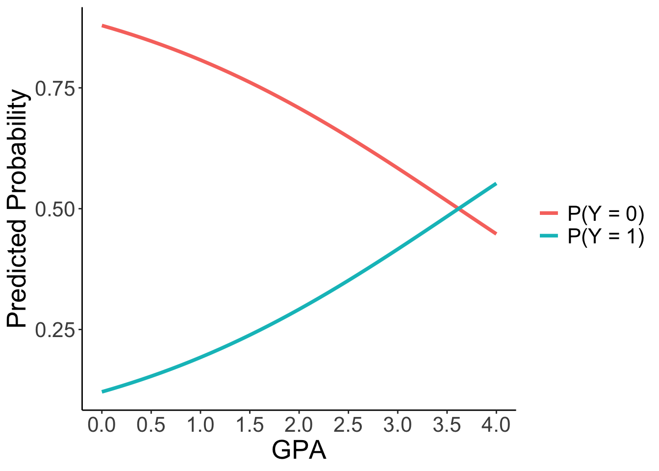
Takehome Note
- For logistic models with two responses:
- Regression weights are now for LOGITS
- The outcome being modeled (Y=0 or Y=1) must be clearly understood
- The change in odds and probability is not linear per unit change in the IV, but instead is linear with respect to the logit
- Interactions will still modify the conditional main effects
- Simple main effects are effects when interacting variables = 0
Exercise: Interpreting Logistic Regression
Below is an R code chunk that simulates a dataset about student study hours and exam outcomes. Your task is to analyze this data.
You are given a dataset exam_data with two variables: study_hours and pass_exam (0 = Fail, 1 = Pass).
Your Tasks:
- Fit a logistic regression model to predict
pass_examfromstudy_hours. - Interpret the intercept (\(\beta_0\)). What are the odds and probability of passing the exam for a student who studied for 0 hours?
- Interpret the slope (\(\beta_1\)). What is the odds ratio associated with a one-hour increase in study time? How does this affect the odds of passing?
Use the R chunk below to write your code.
Here is the solution and interpretation.
Wrap up
Generalized linear models are models for outcomes with distributions that are not necessarily normal
The estimation process is largely the same: maximum likelihood is still the gold standard as it provides estimates with understandable properties
Learning about each type of distribution and link takes time:
- They all are unique and all have slightly different ways of mapping outcome data onto your model
Logistic regression is one of the more frequently used generalized models – binary outcomes are common

ESRM 64503 - Lecture 06: Generalized Linear Models