| id | SATV | SATM |
|---|---|---|
| 1 | 520 | 580 |
| 2 | 520 | 550 |
| 3 | 460 | 440 |
| 4 | 560 | 530 |
| 5 | 430 | 440 |
| 6 | 490 | 530 |
Lecture 07: Matrix Algebra
Matrix Algebra in R
Jihong Zhang, Ph.D.
Educational Statistics and Research Methods (ESRM) Program
University of Arkansas
2024-10-07
Today’s Class
- Matrix Algebra
- Multivariate Normal Distribution
- Multivariate Linear Analysis
Advanced Multivariate Analysis
See the online syllabus here
Recommended for ESRM students and others interested in applied statistics in the social sciences.
A Brief Introduction to Matrices
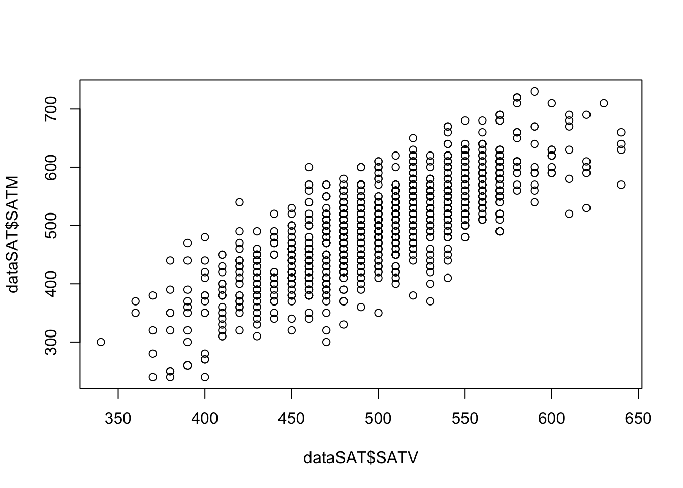
Today’s Example Data
- Imagine that I collected SAT test scores for both the Math (SATM) and Verbal (SATV) sections for 1,000 students.
Last several rows of the data:
Relationship between SATV and SATM:
Background
Matrix operations are fundamental to all modern statistical software.
When you installed R, it also came with required matrix algorithm libraries. Two popular ones are BLAS and LAPACK.
Other optimized libraries include OpenBLAS, AtlasBLAS, GotoBLAS, and Intel MKL.
{bash} Matrix products: default LAPACK: /Library/Frameworks/R.framework/Versions/4.2-arm64/Resources/lib/libRlapack.dylib
From the LAPACK website,
LAPACK is written in Fortran 90 and provides routines for solving systems of simultaneous linear equations, least-squares solutions of linear systems of equations, eigenvalue problems, and singular value problems.
LAPACK routines are written so that as much as possible of the computation is performed by calls to the Basic Linear Algebra Subprograms (BLAS).
Matrix Elements
A matrix (denoted with a capital X) is composed of a set of elements.
- Each element is denoted by its position in the matrix (row and column).
- In R, use
matrix[rowIndex, columnIndex]to extract the element atrowIndexandcolumnIndex.
[1] 3
[1] 5
[1] 3 4
[1] 1 3 5
In statistics, we use \(x_{ij}\) to represent the element in the ith row and jth column. For example, consider a matrix \(\mathbf{X}\) with 1,000 rows and 2 columns:
The first subscript is the index of the rows
The second subscript is the index of the columns
\[ \mathbf{X} = \begin{bmatrix} x_{11} & x_{12}\\ x_{21} & x_{22}\\ \dots & \dots \\ x_{1000, 1} & x_{1000,2} \end{bmatrix} \]
Scalars
A scalar is just a single number
The name scalar is important: the number “scales” a vector—it can make a vector longer or shorter.
Scalars are typically written without boldface:
\[ x_{11} = 520 \]
Each element of a matrix is a scalar.
Matrices can be multiplied by a scalar so that each element is multiplied by that scalar.
Matrix Transpose
- The transpose of a matrix is formed by switching the indices of the rows and columns.
\[ \mathbf{X} = \begin{bmatrix} 520 & 580\\ 520 & 550\\ \vdots & \vdots\\ 540 & 660\\ \end{bmatrix} \]
\[ \mathbf{X}^T = \begin{bmatrix} 520 & 520 & \cdots & 540\\ 580 & 550 & \cdots & 660 \end{bmatrix} \]
An element \(x_{ij}\) in the original matrix \(\mathbf{X}\) becomes \(x_{ji}\) in the transposed matrix \(\mathbf{X}^T\).
Transposes are used to align matrices for operations where the sizes of matrices matter (such as matrix multiplication)
Types of Matrices
Square Matrix: A square matrix has the same number of rows and columns.
- Correlation / covariance matrices are square matrices
Diagonal Matrix: A diagonal matrix is a square matrix with nonzero diagonal elements (\(x_{ij}\neq 0\) for \(i=j\)) and zeros on the off-diagonal elements (\(x_{ij} = 0\) for \(i\neq j\)):
\[ \mathbf{A} = \begin{bmatrix} 2.758 & 0 & 0 \\ 0 & 1.643 & 0 \\ 0 & 0 & 0.879\\ \end{bmatrix} \]
- We will use diagonal matrices to transform correlation matrices into covariance matrices.
Symmetric Matrix: A symmetric matrix is a square matrix where all elements are reflected across the diagonal (\(x_{ij} = x_{ji}\)).
- Correlation and covariance matrices are symmetric matrices
- Question: Is a diagonal matrix always symmetric? True
Linear Combinations
- The addition of a set of vectors (each multiplied by a scalar) is called a linear combination:
\[ \mathbb{y} = a_1x_1 + a_2x_2 + \cdots + a_kx_k = \mathbf{A}^{-1} \mathbf{X} \]
Here, \(\mathbb{y}\) is the linear combination
For all k vectors, the set of all possible linear combinations is called their span
This is typically not emphasized in most analyses—but when working with latent variables it becomes important.
In data, linear combinations occur frequently:
Linear models (i.e., Regression and ANOVA)
Principal components analysis
Question: Do generalized linear models contain linear combinations? True; link function + linear predictor.
Inner (Dot/Cross-) Product of Vectors
An important concept in vector geometry is the inner product of two vectors.
- The inner product is also called the dot product
\[ \mathbf{a} \cdot \mathbf{b} = a_{11}b_{11}+a_{21}b_{21}+\cdots+ a_{N1}b_{N1} = \sum_{i=1}^N{a_{i1}b_{i1}} \]
     [,1]
[1,]    1
[2,]    2
     [,1]
[1,]    2
[2,]    3
     [,1]
[1,]    8
     [,1]
[1,]    8
Using our example data dataSAT,
- In data: the angle between vectors relates to the correlation between variables, and projection relates to regression/ANOVA/linear models.
Combine Two Matrices
Use cbind() to combine by columns and rbind() to combine by rows. Dimensions must be conformable:
cbindrequires the same number of rows.rbindrequires the same number of columns.
Mini Exercise: Dot Product
Compute the dot product of two column vectors and verify it equals the corresponding element of a matrix product.
Define two vectors
a = [1, 3, 5]^Tandb = [2, 4, 6]^Tas3x1matrices.Compute the dot product
a ⋅ bin two ways:
- Using
crossprod(a, b) - Using
t(a) %*% b
- Now form matrices
A = [a a](3x2) andB = [b b](3x2). Computet(A) %*% B. Which entry of this2x2result equalsa ⋅ b?
The dot product is a ⋅ b = 1*2 + 3*4 + 5*6 = 44.
Both crossprod(a, b) and t(a) %*% b return 44.
Forming A = [a a] and B = [b b], the product t(A) %*% B is a 2x2 matrix where every entry equals a ⋅ b = 44, because each entry is the dot product between a column of A and a column of B.
Matrix Algebra
Moving from Vectors to Matrices
A matrix can be thought of as a collection of vectors.
- In R, use
df$[name]ormatrix[, index]to extract a single vector.
- In R, use
Matrix algebra defines a set of operations and entities on matrices.
- I will present a version meant to mirror your previous algebra experiences.
Definitions:
Identity matrix
Zero vector
Ones vector
Basic Operations:
Addition
Subtraction
Multiplication
“Division”
Matrix Addition and Subtraction
Matrix addition and subtraction are much like vector addition and subtraction.
Rules: Matrices must be the same size (rows and columns).
Be careful! R may not produce an error message when adding a matrix and a vector.
Method: the new matrix is constructed by element-by-element addition/subtraction of the previous matrices.
Order: the order of the matrices (pre- and post-) does not matter.
     [,1] [,2]
[1,]    1    2
[2,] 3 4 [,1] [,2]
[1,] 5 6
[2,] 7 8 [,1] [,2]
[1,] 6 8
[2,] 10 12 [,1] [,2]
[1,] -4 -4
[2,] -4 -4Error in `A + C`:
! non-conformable arraysMatrix Multiplication
- The new matrix has the same number of rows as the pre-multiplying matrix and the number of columns as the post-multiplying matrix.
\[ \mathbf{A}_{(r \times c)} \mathbf{B}_{(c\times k)} = \mathbf{C}_{(r\times k)} \]
Rules: The pre-multiplying matrix must have a number of columns equal to the number of rows of the post-multiplying matrix.
Method: the elements of the new matrix consist of the inner (dot) products of the row vectors of the pre-multiplying matrix and the column vectors of the post-multiplying matrix.
Order: The order of the matrices matters.
R: Use the
%*%operator orcrossprodto perform matrix multiplication.
     [,1] [,2] [,3]
[1,]    1    2    3
[2,] 4 5 6 [,1] [,2]
[1,] 5 6
[2,] 7 8
[3,] 9 10 [,1] [,2]
[1,] 46 52
[2,] 109 124 [,1] [,2] [,3]
[1,] 29 40 51
[2,] 39 54 69
[3,] 49 68 87- Example: The inner product of A’s first row vector and B’s first column vector equals AB’s first element.
Mean Centered
\[ X_{(n \times k)}^c = X_{(n \times k)} - I_{(n \times 1)} * \bar{X}_{(1 \times k)} \] where n is the number of cases (sample size) and k is the number of variables.
      Sect1 Sect2
 [1,]  41.4   -20
 [2,]  23.4   -14
 [3,] -16.6   -28
 [4,]  26.4     5
 [5,]  33.4    36
 [6,]   6.4   -31
 [7,] -45.6   -27
 [8,] -26.6    52
 [9,] -11.6    49
[10,] -30.6   -22
Self practice
- Try to mean centered the SATV and SATM of
datSAT. - Store your centered matrix as variable name
X_center - Test your centered matrix using
round(colMeans(X_center), 3)to see if the means are 0s
Identity Matrix
The identity matrix (denoted as \(\mathbf{I}\)) is a matrix that, when pre- or post-multiplied by another matrix, results in the original matrix:
\[ \mathbf{A}\mathbf{I} = \mathbf{A} \]
\[ \mathbf{I}\mathbf{A}=\mathbf{A} \]
The identity matrix is a square matrix that has:
Diagonal elements = 1
Off-diagonal elements = 0
\[ \mathbf{I}_{(3 \times 3)} = \begin{bmatrix} 1&0&0\\ 0&1&0\\ 0&0&1\\ \end{bmatrix} \]
R: Create an identity matrix using the
diag()function.
Zero and One Vector
The zero and one vectors are column vectors of zeros and ones, respectively:
\[ \mathbf{0}_{(3\times 1)} = \begin{bmatrix}0\\0\\0\end{bmatrix} \]
\[ \mathbf{1}_{(3\times 1)} = \begin{bmatrix}1\\1\\1\end{bmatrix} \]
When pre- or post-multiplied with a matrix (\(\mathbf{A}\)), the result with the zero vector is:
\[ \mathbf{A0=0} \]
\[ \mathbf{0^TA=0} \]
R:
Matrix “Division”: The Inverse Matrix
Division from algebra:
First: \(\frac{a}{b} = b^{-1}a\)
Second: \(\frac{a}{b}=1\)
“Division” in matrices serves a similar role.
For square symmetric matrices, an inverse matrix is a matrix that, when pre- or post-multiplied with another matrix, produces the identity matrix:
\[ \mathbf{A^{-1}A=I} \]
\[ \mathbf{AA^{-1}=I} \]
R: Use
solve()to calculate the matrix inverse.
     [,1] [,2] [,3]
[1,]    1    0    0
[2,]    0    1    0
[3,] 0 0 1- Caution: The calculation is complicated; even computers can struggle. Not all matrices can be inverted:
Example: The Inverse of the Variance–Covariance Matrix
In data analysis, the inverse shows up constantly in statistics.
- Models that assume some form of (multivariate) normality need an inverse covariance matrix.
Using our SAT example:
Our data matrix has size (\(1000\times 2\)), which is not invertible.
However, \(\mathbf{X^TX}\) has size (\(2\times 2\))—square and symmetric.
SATV SATM SATV 251797800 251928400 SATM 251928400 254862700- The inverse \(\mathbf{(X^TX)^{-1}}\) is:
Matrix Algebra Operations
\(\mathbf{(A+B)+C=A+(B+C)}\)
\(\mathbf{A+B=B+A}\)
\(c(\mathbf{A+B})=c\mathbf{A}+c\mathbf{B}\)
\((c+d)\mathbf{A} = c\mathbf{A} + d\mathbf{A}\)
\(\mathbf{(A+B)^T=A^T+B^T}\)
\((cd)\mathbf{A}=c(d\mathbf{A})\)
\((c\mathbf{A})^{T}=c\mathbf{A}^T\)
\(c\mathbf{(AB)} = (c\mathbf{A})\mathbf{B}\)
\(\mathbf{A(BC) = (AB)C}\)
- \(\mathbf{A(B+C)=AB+AC}\)
- \(\mathbf{(AB)}^T=\mathbf{B}^T\mathbf{A}^T\)
Advanced Matrix Functions/Operations
We end our matrix discussion with some advanced topics.
To help us throughout, consider the correlation matrix of our SAT data:
          SATV      SATM
SATV 1.0000000 0.7752238
SATM 0.7752238 1.0000000
\[ R = \begin{bmatrix}1.00 & 0.78 \\ 0.78 & 1.00\end{bmatrix} \]
Matrix Trace
For a square matrix \(\mathbf{A}\) with p rows/columns, the matrix trace is the sum of the diagonal elements:
\[ tr\mathbf{A} = \sum_{i=1}^{p} a_{ii} \]
In R, we can use
tr()inpsychpackage to calculate matrix traceFor our data, the trace of the correlation matrix is 2
For all correlation matrices, the trace is equal to the number of variables
The trace is considered as the total variance in multivariate statistics
- Used as a target to recover when applying statistical models
Model Determinants
A square matrix can be characterized by a scalar value called a determinant:
\[ \text{det}\mathbf{A} =|\mathbf{A}| \]
Manual calculation of the determinant is tedious. In R, we use
det()to calculate matrix determinantThe determinant is useful in statistics:
Shows up in multivariate statistical distributions
Is a measure of “generalized” variance of multiple variables
If the determinant is positive, the matrix is called positive definite → the matrix has an inverse
If the determinant is zero, the matrix is called singular matrix → the matrix does not have an inverse, cannot used for multivariate analysis.
If the determinant is not positive, the matrix is called non-positive definite → the matrix has an inverse but very rare in multivariate analysis, maybe due to the mistakes in your data.
Mini Exercise 2: Inverse Model with Positive Determinant
Wrap Up
Matrices show up nearly anytime multivariate statistics are used, often in the help/manual pages of the package you intend to use for analysis
You don’t have to do matrix algebra, but please do try to understand the concepts underlying matrices
Your working with multivariate statistics will be better off because of even a small amount of understanding
Multivariate Normal Distribution
Covariance and Correlation in Matrices
The covariance matrix \(\mathbf{S}\) is found by:
\[ \mathbf{S}=\frac{1}{N-1} \mathbf{(X-1\cdot\bar x^T)^T(X-1\cdot\bar x^T)} \]
SATV SATM SATV 2479.817 3135.359 SATM 3135.359 6596.303SATV SATM SATV 2479.817 3135.359 SATM 3135.359 6596.303
From Covariance to Correlation
- If we take the SDs (the square root of the diagonal of the covariance matrix) and put them into diagonal matrix \(\mathbf{D}\), the correlation matrix is found by:
\[ \mathbf{R = D^{-1}SD^{-1}} \] \[ \mathbf{S = DRD} \]
         SATV     SATM
SATV 2479.817 3135.359
SATM 3135.359 6596.303 [,1] [,2]
[1,] 49.79777 0.00000
[2,] 0.00000 81.21763 [,1] [,2]
[1,] 1.0000000 0.7752238
[2,] 0.7752238 1.0000000 SATV SATM
SATV 1.0000000 0.7752238
SATM 0.7752238 1.0000000Generalized Variance
- The determinant of the covariance matrix is called generalized variance
\[ \text{Generalized Sample Variance} = |\mathbf{S}| \]
It is a measure of spread across all variables
Reflecting how much overlapping area (covariance) across variables relative to the total variances occurs in the sample
Amount of overlap reduces the generalized sample variance
[1] 6527152 SATV SATM
SATV 2479.817 0.000
SATM 0.000 6596.303[1] 16357628[1] 0.399028 SATV SATM
SATV 2479.817 16357628.070
SATM 16357628.070 6596.303[1] -2.67572e+14The generalized sample variance is:
- Largest when variables are uncorrelated
- Zero when variables from a linear dependency
Total Sample Variance
The total sample variance is the sum of the variances of each variable in the sample.
- The sum of the diagonal elements of the sample covariance matrix.
- The trace of the sample covariance matrix.
\[ \text{Total Sample Variance} = \sum_{v=1}^{V} s^2_{x_i} = \text{tr}\mathbf{S} \]
Total sample variance for our SAT example:
The total sample variance does not take into consideration the covariances among the variables.
- It will not equal zero if linear dependency exists.
Multivariate Normal Distribution and Mahalanobis Distance
- The PDF of the multivariate normal distribution is very similar to the univariate normal distribution.
\[ f(\mathbf{x}_p) = \frac{1}{(2\pi)^{\frac{V}2}|\mathbf{\Sigma}|^{\frac12}}\exp[-\frac{\color{tomato}{(x_p^T - \mu)^T \mathbf{\Sigma}^{-1}(x_p^T-\mu)}}{2}] \]
Where \(V\) represents the number of variables and the highlighted term is the Mahalanobis distance.
We use \(MVN(\mathbf{\mu, \Sigma})\) to represent a multivariate normal distribution with mean vector \(\mathbf{\mu}\) and covariance matrix \(\mathbf{\Sigma}\).
Similar to the squared error in the univariate case, we can calculate the squared Mahalanobis distance for each observed individual in the context of a multivariate distribution.
\[ d^2(x_p) = (x_p^T - \mu)^T \Sigma^{-1}(x_p^T-\mu) \]
- In R, we can use
mahalanobiswith a data vector (x), mean vector (center), and covariance matrix (cov) to calculate the squared Mahalanobis distance for one individual.
SATV SATM
520 580 [1] 1.346228[1] 0.4211176[1] 0.6512687 [,1]
[1,] 1.346228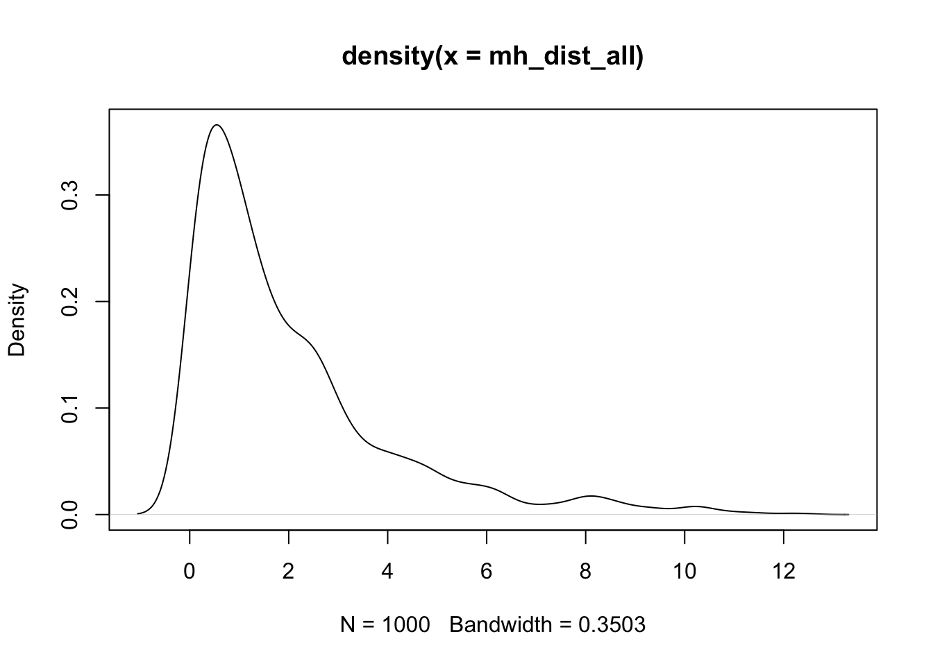
Multivariate Normal Properties
The multivariate normal distribution has useful properties that appear in statistical methods:
If \(\mathbf{X}\) is distributed multivariate normally:
- Linear combinations of \(\mathbf{X}\) are normally distributed
- All subsets of \(\mathbf{X}\) are multivariate normally distributed
- A zero covariance between a pair of variables of \(\mathbf{X}\) implies that the variables are independent
- Conditional distributions of \(\mathbf{X}\) are multivariate normal
How to Use the Multivariate Normal Distribution in R
Similar to other distribution functions, use dmvnorm to get the density given the observations and the parameters (mean vector and covariance matrix). rmvnorm generates multiple samples from the distribution.
  SATV   SATM
499.32 498.27 SATV SATM
SATV 2479.817 3135.359
SATM 3135.359 6596.303[1] 3.177814e-05[1] 5.046773e-05[1] -10682.62| SATV | SATM |
|---|---|
| 563.5026 | 631.6245 |
| 499.0337 | 507.6084 |
| 445.5664 | 460.9351 |
| 502.6223 | 580.6672 |
| 449.6527 | 352.2973 |
| 450.7611 | 469.3925 |
| 491.3205 | 481.4378 |
| 567.1666 | 636.8755 |
| 443.9740 | 419.2099 |
| 504.9611 | 513.8619 |
| 443.7179 | 426.9764 |
| 441.1004 | 370.3551 |
| 439.0337 | 448.5081 |
| 545.1352 | 567.4855 |
| 563.2110 | 567.7634 |
| 553.4351 | 616.0691 |
| 518.5158 | 562.1784 |
| 428.6370 | 414.4879 |
| 563.2217 | 608.2384 |
| 500.1564 | 432.5149 |
Mini Exercise 3: Self Practice
Using a small practice matrix and the tools from this lecture, complete the following steps. Fill in the underlined placeholders where indicated.
- Build the data matrix
Xwith columnsSATVandSATM(as a numeric matrix). Compute:
- The sample mean vector
XBARand covariance matrixS. - The correlation matrix
Rand its tracetr(R).
- Verify basic matrix operations:
- Center
XtoXc = X - ____ %*% t(____)using a ones vector and the mean vector. - Check that
colMeans(Xc)is (approximately) ____. - Confirm
t(Xc) %*% Xc / (____ - 1)equals ____.
- Work with products and inverses:
- Compute
XtX = crossprod(____)and its inverseXtX_inv = solve(____). - Verify
round(XtX_inv %*% ____, 6)equals the identity.
- Mahalanobis distances and MVN:
- Compute squared Mahalanobis distances for all rows of
Xusingmahalanobiswith center____and cov____. - Plot the density of the distances.
XBARis the 2x1 mean vector ofSATVandSATM;Sis their 2x2 sample covariance matrix;Ris the correlation matrix andtr(R)equals the sum of its diagonal (2.0 for perfectly standardized variables; here it depends on scaling).- Centering with a ones vector yields
colMeans(Xc)approximately zero; andt(Xc) %*% Xc / (n - 1)equalsSby definition of sample covariance. XtX_inv %*% XtXequals the identity (up to rounding) whenXtXis invertible.mahalanobis(X, XBAR, S)returns squared distances used in multivariate normal contexts; the density plot visualizes their distribution.
Wrapping Up
We are now ready to discuss multivariate models and the art/science of multivariate modeling.
Many of the concepts from univariate models carry over:
- Maximum likelihood
- Model building via nested models
- Concepts involving multivariate distributions
Matrix algebra was necessary to concisely describe our distributions (which will soon be models).
Understanding the multivariate normal distribution is essential, as it is the most commonly used distribution for estimating multivariate models.
Next class, we will return to data analysis—for multivariate observations—using R’s lavaan package for path analysis.

ESRM 64503 - Lecture 07: Matrix Algebra