Lecture 08: Block Design II
Experimental Design in Education
2025-03-07
Example 2: Tutoring session
- Let’s look at a simple example:
- Research question: What is the effect of time of day (morning session vs. afternoon session) of tutoring session on midterm grades?
- The Primary Investigator (PI) of the study wants to control for different tutor(s), believing some tutors may be better than others. Thus, they design a completely randomized block design.
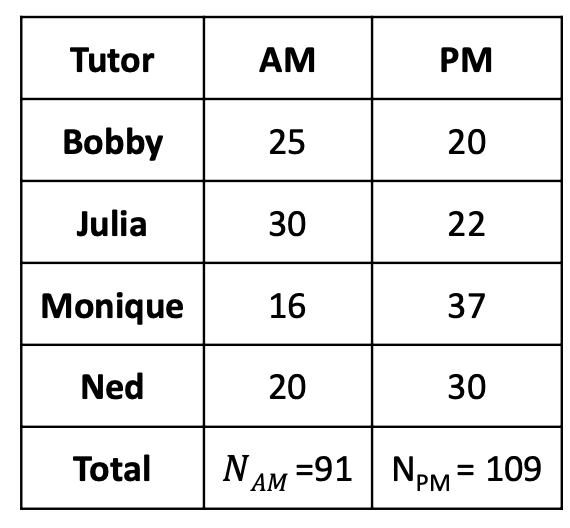
- Each tutor works with students in the morning and afternoon.
- In this example, student select their favorite tutor, but are then randomly assigned to either a morning (AM) or afternoon (PM) session.
- 200 total students: 91 in the morning, 109 in the afternoon
Note
DV: Midterm Score (in cells)
Variables and Null Hypothesis
- IV: Time (a = 2 )
- 2 levels: AM and PM
- Nuisance factor: Tutor (b = 4 )
- 4 levels: Booby, Julia, Monique, and Ned
- DV: Midterm Score
- Null hypothesis pertaining to the IV of interest:
- \(H_0:\mu_{𝐴𝑀} = \mu_{𝑃𝑀} → a= 2\)
- We will also have a null hypothesis pertaining to the blocking factor:
- \(H_0:\mu_{Bobby} = \mu_{Julia} = \mu_{Monique} =\mu_{Ned} → b=4\)
- Two Nulls = two values of \(F_{obs}\), two values of \(F_{crit}\), two decisions
Note
DV: Midterm Score (in cells)
Sum of Squares
IV: Time (𝑎= 2 )
Nuisance factor: Tutor (𝑏= 4 )
DV: Midterm Score
Now:
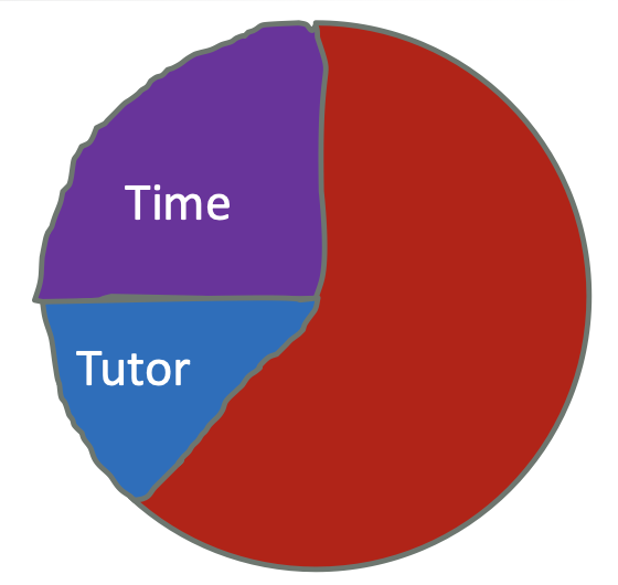
- \(𝑆𝑆_{Total} =\color{red}{𝑆𝑆_{𝑀𝑜𝑑𝑒𝑙}}+\color{purple}{𝑆𝑆_{𝐵𝑙𝑜𝑐𝑘}}+\color{blue}{𝑆𝑆_{𝐸𝑟𝑟𝑜𝑟}}\)
Thus, we can partition the effects into three parts:
Sum of squares due to treatments (IV = Time),
Sum of squares due to the blocking factor,
and Sum of squares due to error.
We do not model an interaction with blocked designs. (we will talk about it later.)
Mean of Squares and F-statistics
- IV: Time (𝑎= 2 )
- Nuisance factor: Tutor (𝑏= 4 )
- DV: Midterm Score
- Model: \(𝑆𝑆_{Total} =\color{red}{𝑆𝑆_{𝑀𝑜𝑑𝑒𝑙}}+\color{purple}{𝑆𝑆_{𝐵𝑙𝑜𝑐𝑘}}+\color{blue}{𝑆𝑆_{𝐸𝑟𝑟𝑜𝑟}}\)
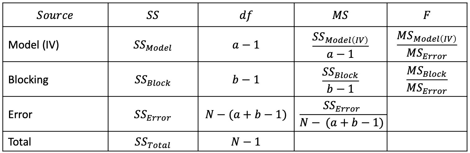
- ANOVA table:
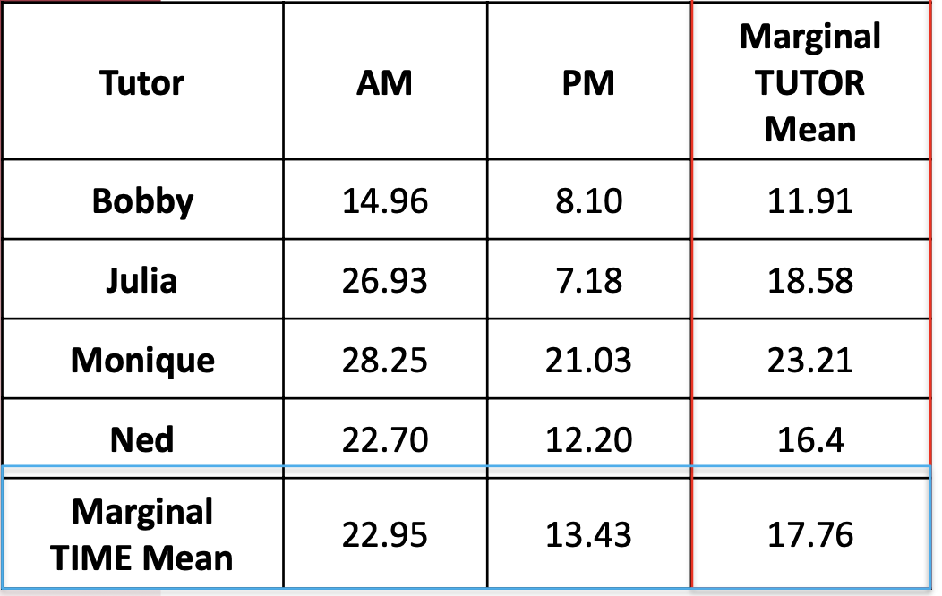
Marginal Means
- A marginal mean is the mean for one level of the variable, ignoring the other variable
For example:
- The AM marginal mean is the average of all students’ midterm scores in the morning, ignoring who they have as a tutor \[ \bar{y}_{AM.} = 22.95 \]
- The Bobby marginal mean is the average of all students’ midterm scores who had Bobby as a tutor, ignoring time of day \[ \bar{y}_{.Bobby} = 11.91 \]
Results of ANOVA Table
- Then, we can fill out the ANOVA table:
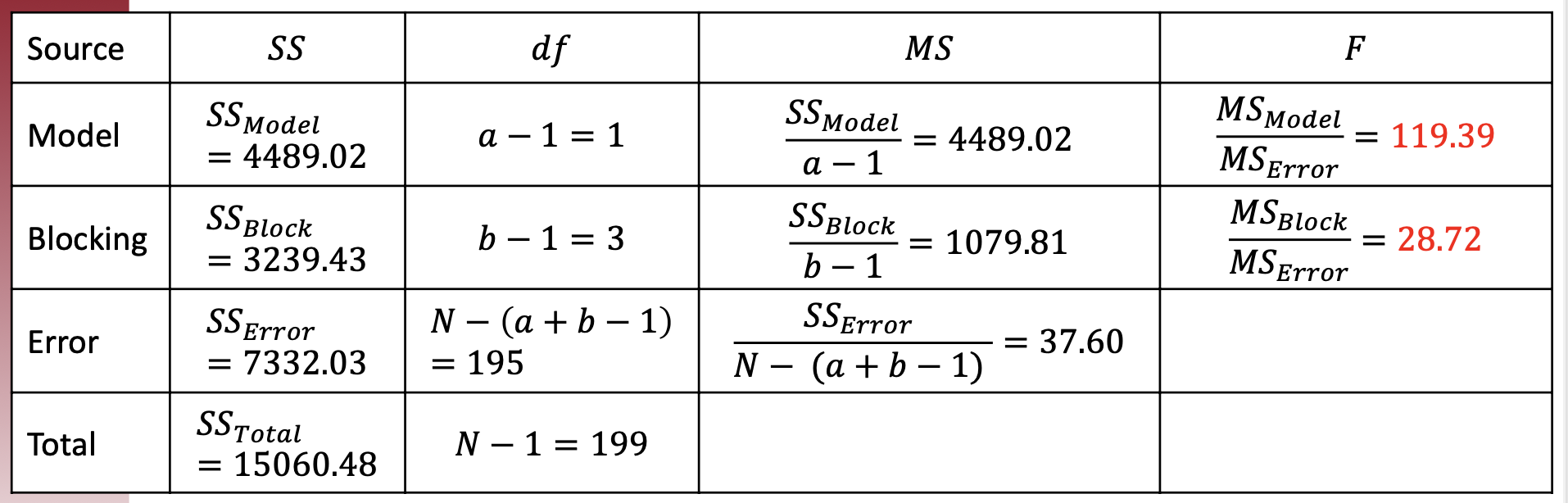
Note
Under \(\alpha=.05\), for “Model” factor – Time, we have \(df_{Model}\) = 1, \(df_{error} = 195\): \(F_{crit}=3.89\) so sig.
Similarly, for “Blocking” - Tutor, we have \(df_{block}\) = 3, \(df_{error} = 195\): \(F_{crit}=2.65\) so sig.
Example 4: Hours spent on the study in varied environments
- Background: Comparing the hours spent on the study for gender (male and female) blocks in different environments (at home and at college). To represent this experiment in the figure will be as follows:
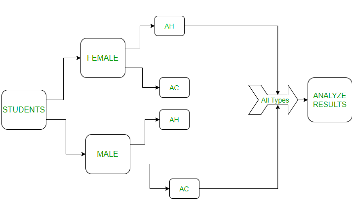
- Where AC: At College, AH: At Home
    y gender env
1 5.5   male  ah
2 5.0   male  ac
3 4.0 female  ah
4 6.2 female acTry to obtain (1) the sum of squares for treatment and block (2) F-statistics. Then, interpret the results.
            Df Sum Sq Mean Sq F value Pr(>F)
gender       1 0.0225  0.0225   0.012  0.930
env          1 0.7225  0.7225   0.396  0.642
Residuals 1 1.8225 1.8225 - Explanation: The value of Mean Sq is
0.7225<<1.8225,i.e, here blocking wasn’t necessary. And as Pr value is 0.642 > 0.05 (5% significance) we fail to reject the null hypothesis - there is no sufficient evidence suggesting females and males have significant differences in performance.