or \(H_0: \mu_{A_1B_1}-\mu_{A_2B_1}=\mu_{A_1B_2}-\mu_{A_2B_2}\)
B’s group differences do not change at different levels of A. OR A’s group differences do not change at different levels of B.
Hypothesis testing for two-way ANOVA (III)
Example
Background: A researcher is investigating how study method (Factor A: Lecture vs. Interactive) and test format (Factor B: Multiple-Choice vs. Open-Ended) affect student performance (dependent variable: test scores). The study involves randomly assigning students to one of the two study methods and then assessing their performance on one of the two test formats.
Main Effect of Study Method (Factor A):
H0: There is no difference in test scores between students who used the Lecture method and those who used the Interactive method.
H1: There is a significant difference in test scores between the two study methods.
Main Effect of Test Format (Factor B):
H0: There is no difference in test scores between students taking a Multiple-Choice test and those taking an Open-Ended test.
H1: There is a significant difference in test scores between the two test formats.
Interaction Effect (Study Method × Test Format):
H0: The effect of study method on test scores is the same regardless of test format.
H1: The effect of study method on test scores depends on the test format (i.e., there is an interaction).
Hypothesis testing for two-way ANOVA (IV)
Example: Tutoring Program and Types of Schools on Grades
IVs:
Tutoring Programs: (1) No tutor; (2) Once a week; (3) Daily
Types of schools: (1) Public (2) Private-secular (3) Private-religious
Research purpose: to examine the effect of tutoring program (no tutor, once a week, and daily) AND types of school (e.g., public, private-secular, and private-religious) on the students’ grades
Question: What are the null and alternative hypotheses for the main effects in the example?:
Factor A’s Main effect: “Controlling school types, are there differences in the students’ grade across three tutoring programs?”
library(tidyverse)# Set seed for reproducibilityset.seed(123)# Define sample size per groupn <-30# Define factor levels
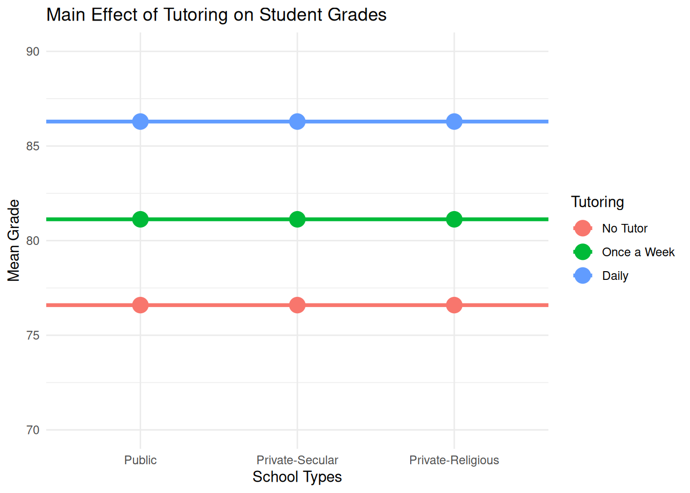
tutoring <-rep(c("No Tutor", "Once a Week", "Daily"), each =3* n)school <-rep(c("Public", "Private-Secular", "Private-Religious"), times = n *3)# Simulate student grades with assumed effectsgrades <-c(rnorm(n, mean =75, sd =5), # No tutor, Publicrnorm(n, mean =78, sd =5), # No tutor, Private-Secularrnorm(n, mean =76, sd =5), # No tutor, Private-Religiousrnorm(n, mean =80, sd =5), # Once a week, Publicrnorm(n, mean =83, sd =5), # Once a week, Private-Secularrnorm(n, mean =81, sd =5), # Once a week, Private-Religiousrnorm(n, mean =85, sd =5), # Daily, Publicrnorm(n, mean =88, sd =5), # Daily, Private-Secularrnorm(n, mean =86, sd =5) # Daily, Private-Religious)# Create a dataframedata <-data.frame(Tutoring =factor(tutoring, levels =c("No Tutor", "Once a Week", "Daily")),School =factor(school, levels =c("Public", "Private-Secular", "Private-Religious")),Grades = grades)
Main effect of Tutoring Programs
Collapsing across School Type
Ignoring the difference levels of School Type
Averaging DV regarding Tutoring Programs across the levels of School Type
Main effect of School Type
Collapsing across Tutoring Program
Ignoring the difference levels of Tutoring Program
Averaging DV regarding School Type across the levels of Tutoring Programs
Ignoring the effect of school types, we can tell the main effect of tutor programs on students’ grades (Daily tutoring has the highest grade, followed by once a week).
Code
# Compute mean and standard error for each tutoring grouptutoring_summary <- data |>group_by(Tutoring) |>summarise(Mean_Grade_byTutor =mean(Grades),School =factor(c("Public","Private-Secular", "Private-Religious"), levels =c("Public","Private-Secular", "Private-Religious")) ) school_summary <- data |>group_by(School) |>summarise(Mean_Grade_bySchool =mean(Grades) ) total_summary <- tutoring_summary |>left_join(school_summary, by ="School")# Plot main effect of tutoringggplot(total_summary, aes(x = School)) +geom_point(aes(y = Mean_Grade_byTutor, color = Tutoring), size =5) +geom_hline(aes(yintercept = Mean_Grade_byTutor, color = Tutoring), linewidth =1.3) +scale_y_continuous(limits =c(70, 90), breaks =seq(70, 90, 5)) +labs(title ="Main Effect of Tutoring on Student Grades",x ="School Types",y ="Mean Grade") +theme_minimal()
There variance components (random effects) included in a full two-way ANOVA with two Factors.
Model 2: Visualization of Two-Way ANOVA with Interaction
In the graph:
There is the LARGE effect of Factor A and very small effect of Factor B:
Effect of Factor A: the LARGE distance between two green stars
Effect of Factor B: the very small distance between two red stars
In the graph, there is an intersection between two lines → This is an interaction effect between two factors!
The level of Factor B depends upon the level of Factor A – B1 is higher than B2 for A1, but lower for A2 – B2 is lower than B1 for A1, but higher for A2
Main Effect A: Ignoring type of school, are there differences in grades across type of tutoring?
Under alpha=.05 level, because F-observed (F_observed=89.065) exceeds the critical value (p < .001), we reject the null that all means are equal across tutoring type (ignoring the effect of school type).
There is a significant main effect of tutoring type on grade.
Main Effect B: Ignoring tutoring type, are there differences in grades across type of school?
Under alpha=.05 level, because F-observed (F_observed=95.40) exceeds the critical value (p = .453), we retain (or fail to reject) the null hypothesis that all means are equal across school type (ignoring the effect of tutoring type).
There is no evidence suggesting a significant main effect of school type on grade.
Interaction Effect: Does the effect of tutoring type on grades depend on the type of school?
Under alpha=.05 level, because F-observed (F_observed=2.21) does not exceed the critical value (p = 0.102), we fail to reject the null that the effect of Factor A depends on Factor B.
There is not a significant interaction between tutoring type and school type on grades.
Assumptions for conductiong 2-way ANOVA
In order to compare our sample to the null distribution, we need to make sure we are meeting some assumptions for each CELL:
Variance of DV in each cell is about equal. → Homogeneity of variance
DV is normally distributed within each cell. → Normality
Observations are independent. → Independency
Robustness of assumption violations:
Violations of independence assumption: bad news! → Not robust to this!
Having a large N and equal cell sizes protects you against violations of the normality assumption → Rough suggestion: have at least 15 participants per cell → If you don’t have large N or equal groups, check cell normality 2 ways: (1) skew/kurtosis values, (2) histograms
Use Levene’s test to check homogeneity of cell variance assumption → If can’t assume equal variances, use Welch or Brown-Forsyth. → However, F is somewhat robust to violations of HOV as long as within-cell standard deviations are approximately equal.
Two-way ANOVA: Calculation based on Grand & Marginal & Cell Means
This research study is an adaptation of Gueguen (2012) described in Andy Field’s text. Specifically, the researchers hypothesized that people with tattoos and piercings were more likely to engage in riskier behavior than those without tattoos and piercings. In addition, the researcher wondered whether this difference varied, depending on whether a person was male or female.
Question: How many IVs? How many levels for each.
Answer: 2 IVs: (1) Whether or not having Tattos and Piercings (2) Male of Female. DV: Frequency of risk behaviors
Data input in R
Either you can import a CSV file, or manually import the data points (for small samples).
# Df Sum Sq Mean Sq F value Pr(>F)
# gender 1 7.84 7.840 2.942 0.112
# tatto_piercing 1 28.09 28.090 10.540 0.007 **
# gender:tatto_piercing 1 1.69 1.690 0.634 0.441
# Residuals 12 31.98 2.665
Main Effect of Tattoo-Piercing: Reject the null → Ignoring the gender, there is a significant main effect of tattoo on risky behavior.
Main Effect of Gender: Retain the null → Ignoring the tattoo, there is NO significant main effect of gender on risky behavior.
Interaction: Retain the null → Under alpha=.05 level, because F-observed (F=0.63) does not exceed the critical value (F=4.75), we fail to reject the null that the effect of Factor A depends on Factor B. → “There is NO significant interaction between gender and tattoo on risky behavior.”
ShinyApp for ANOVA
Other extensions about 2-way ANOVA: I
Type I? Type II? Type III?
Effect sums of squares (SSA, SSB, SSAB) are a decomposition of the total sum of squared deviations from the overall mean (SST).
How the SST is decomposed depends on characteristics of the data as well as the hypotheses of interest to the researcher.
Type I sums of squares (SS) are based on a sequential decomposition.
For example, if your ANOVA model statement is “MODEL Y = A B A*B”, then, the sum of squares are considered in effect order A, B, A*B, with each effect adjusted for all preceding effects in the model.
Thus, any variance that is shared between the various effects will be sub-summed by the variable entered earlier.
Pros:
Nice property: balanced or not, SS for all the effects add up to the total SS, a complete decomposition of the predicted sums of squares for the whole model. This is not generally true for any other type of sums of squares.
Preferable when some factors (such as nesting) should be taken out before other factors. For example, with unequal number of male and female, factor “gender” should precede “subject” in an unbalanced design.
Cons: 1. Order matters! 2. Not appropriate for factorial designs, but might be ok for Blocking designs.
Other extensions about 2-way ANOVA: II
With Type II SS, each main effect is considered as though it were added after the other main effects but before the interaction.
Any interaction effects are calculated based on a model already containing the main effects.
Any variance that is shared between A and B is not considered part of A or B.
Thus, interaction variance that is shared with A or with B will be counted as part of the main effect, and not as part of the interaction effect.
Pros:
appropriate for model building, and natural choice for regression
most powerful when there is no interaction
invariant to the order in which effects are entered into the model
Cons:
For factorial designs with unequal cell samples, Type II sums of squares test hypotheses that are complex functions of the cell ns that ordinarily are not meaningful.
Not appropriate for factorial designs.
Other extensions about 2-way ANOVA: III
Type III SS considers all effects as though they are added last.
Any shared variance ends up not being counted in any of the effects.
In ANOVA, when the data are balanced (equal cell sizes) and the factors are orthogonal and all three types of sums of squares are identical.
Orthogonal, or independent, indicates that there is no variance shared across the various effects, and the separate sums of squares can be added to obtain the model sums of squares.
Pros:
Not sample size dependent: effect estimates are not a function of the frequency of observations in any group (i.e., for unbalanced data, where we have unequal numbers of observations in each group).
Cons:
Not appropriate for designs with missing cells: for ANOVA designs with missing cells, Type III sums of squares generally do not test hypotheses about least squares means, but instead test hypotheses that are complex functions of the patterns of missing cells in higher-order containing interactions and that are ordinarily not meaningful.
In general, for the factorial design, we usually report Type III SS, unless you have missing cells in your model.
Final discussion
In this example,
The interaction effect shows several issues:
Violation of independency assumption
Violation of normality assumption in the condition of “Male” and “Tattoo=Yes”
We can guess/think about one possibility that it might be cause by several reasons. (e.g., too small sample sizes, not randomized assignments of the samples, not a significant interaction effect, etc.)
From the two-way ANOVA results, we found that the interaction effect is not significant.
Thus, in this case, it is more reasonable to conduct
one-way ANOVA for “Group” variable, and
one-way ANOVA for “Gender” variable, separately.
For each of one-way ANOVAs, we should check the assumptions, conduct one-way ANOVA, and post-hoc test separately as well.