Lecture 12: ANCOVA
Experimental Design in Education
2025-04-09
ANCOVA: Example
We are interested in
Comparing the method of instruction on students’ mathematical problem‑solving performance, as measured by a test score.
- The test is composed of word problems that are each presented in a few sentences.
- Ex: “Joe buys 60 cantaloupes and sells 5. He then gives away 4…”
- DV = number of problems correctly answered in an hour.
- IV = method of instruction (three levels)
- The test is composed of word problems that are each presented in a few sentences.
One-way, independent ANOVA: If the omnibus F is significant, we conclude that the instructional methods differ in the mean number of correctly answered problems.
But, performance on math word problems may be affected by factors beyond instructional method and math ability.
- To name a few: academic motivation scores, verbal proficiency scores, hunger ratings, previous years’ math grades…
The DV score results from instructional method + the other factors we just listed.
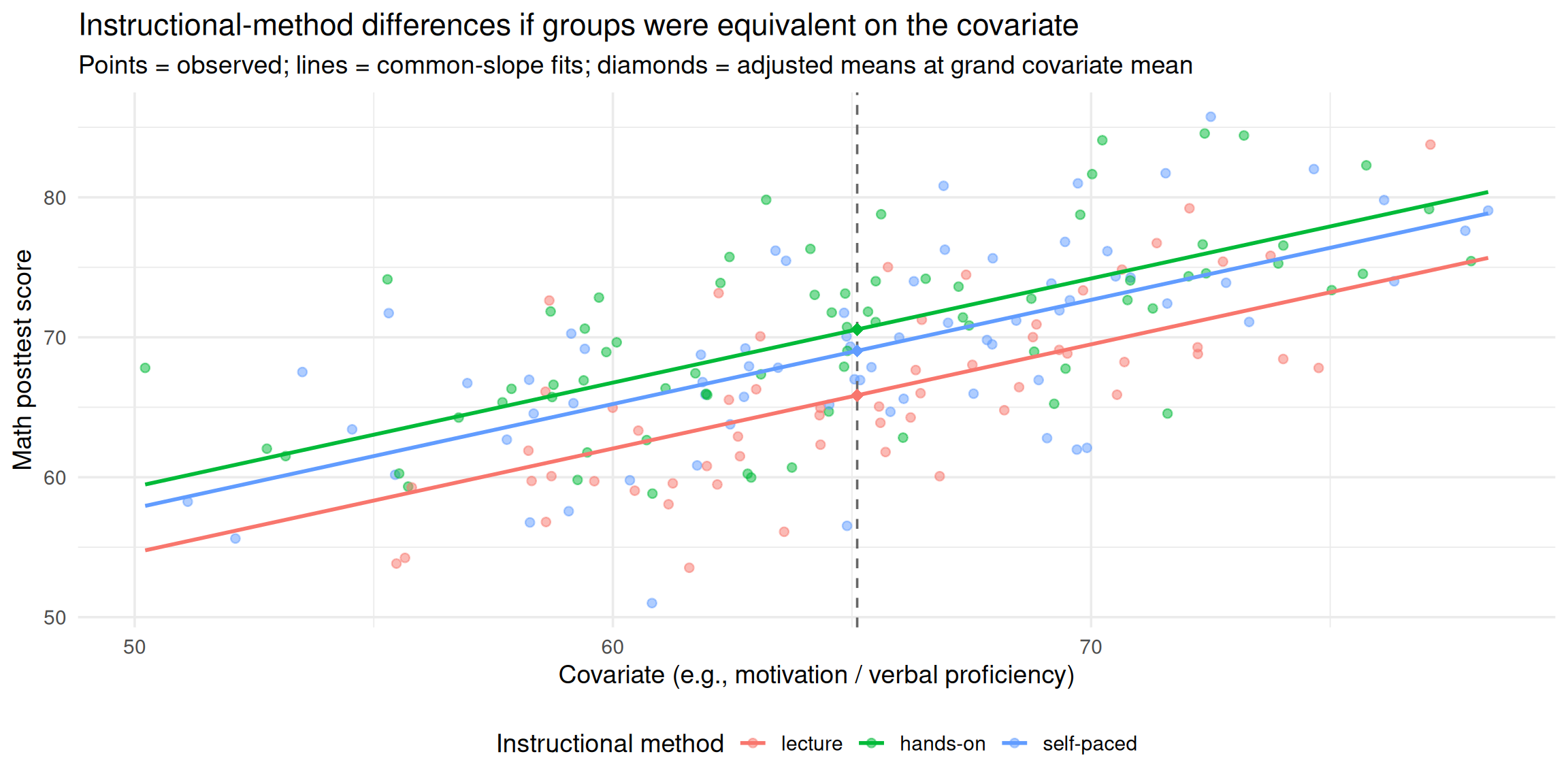
We really want to ask:
To what extent would we have observed instructional‑method differences in math scores if the groups had been equivalent in motivation (or verbal proficiency)?
By looking over the plot, we can find that there is a general linear relationship (i.e., straight line) between the covariate (pretest) and the DV (mathtest).
R code to check linear relationship
# Plot
ggplot(df, aes(x = pretest, y = posttest)) +
  geom_point(color = "blue", alpha = 0.6) +
  geom_smooth(method = "lm", color = "steelblue", se = FALSE) +
  theme_minimal(base_size = 14) +
  labs(x = "pretest", y = "mathtest") +
  theme(legend.position = "bottom") +
  guides(color = guide_legend(title = NULL))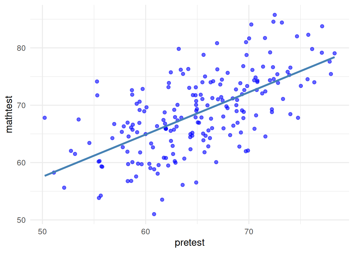
Example Python code to check homogeneity of regression slope
import matplotlib.pyplot as plt
import numpy as np

# Generate x values (covariate)
x = np.linspace(0, 10, 100)

# Homogeneous regression slopes
y1_homo = 1.0 * x + 2
y2_homo = 1.0 * x + 4
y3_homo = 1.0 * x + 6

# Heterogeneous regression slopes
y1_hetero = -0.1 * x + 6
y2_hetero = 1.2 * x + 1
y3_hetero = 0.9 * x + 3

# Create the figure with two subplots
fig, axs = plt.subplots(1, 2, figsize=(12, 5), sharey=True)

# Plot for homogeneous regression slopes
axs[0].plot(x, y1_homo, label="Group 1")
axs[0].plot(x, y2_homo, label="Group 2")
axs[0].plot(x, y3_homo, label="Group 3")
axs[0].set_title("(a) Homogeneity of regression (slopes)")
axs[0].set_xlabel("Covariate (X)")
axs[0].set_ylabel("DV (Y)")
axs[0].legend()

# Plot for heterogeneous regression slopes
axs[1].plot(x, y1_hetero, label="Group 1")
axs[1].plot(x, y2_hetero, label="Group 2")
axs[1].plot(x, y3_hetero, label="Group 3")
axs[1].set_title("(b) Heterogeneity of regression (slopes)")
axs[1].set_xlabel("Covariate (X)")
axs[1].legend()

plt.tight_layout()
plt.show()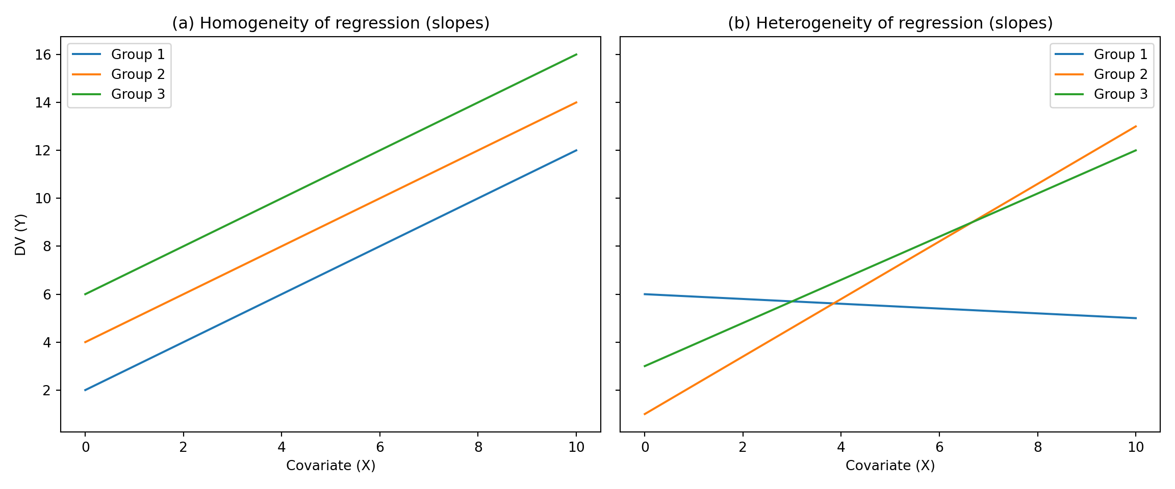
ANCOVA: Assumption Check V
- Assumption Check in ANCOVA:
- Homogeneity of Regression Slope:
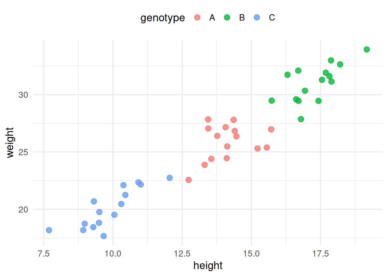
When we visually inspect the three regression slopes (covariate predicting the DV), the relationships appear approximately equal.
R code to check homogeneity of regression slope
# Plot
ggplot(df, aes(x = pretest, y = posttest, color = method)) +
  geom_point(alpha = 0.6) +
  geom_smooth(method = "lm", se = FALSE) +
  scale_color_manual(values = c("steelblue", "tomato", "seagreen4")) +
  theme_minimal(base_size = 14) +
  labs(x = "pretest", y = "mathtest") +
  theme(legend.position = "bottom") +
  guides(color = guide_legend(title = NULL))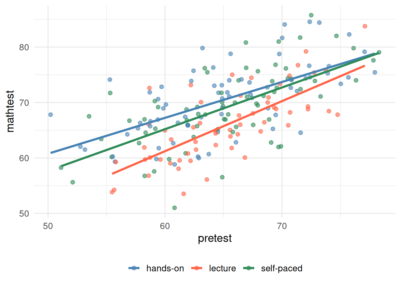
Visualization
Based on the adjusted means, pretest, and posttest means, we can visualize the results using a bar plot.
Code
used_colors <- c("steelblue", "tomato", "seagreen4")
used_group_labels <- c("Pretest", "Posttest", "Adjusted")
results2 |>
  select(method, pretest_mean, posttest_mean, adjusted_mean) |>
  pivot_longer(ends_with("_mean"), names_to = "type", values_to = "Mean") |>
  mutate(type = factor(type, levels = paste0(c("pretest", "posttest", "adjusted"), "_mean"))) |>
  ggplot(aes(y = method, x = Mean)) +
  geom_col(aes(y = method, x = Mean, fill = type), position = position_dodge()) +
  geom_text(aes(x = Mean + 5, label = round(Mean, 2), color = type), position = position_dodge(width = .85)) +
  scale_color_manual(values = used_colors, labels = used_group_labels) +
  scale_fill_manual(values = used_colors, labels = used_group_labels) +
  labs(y = "", title = "Comparing Adjusted and Unadjusted Means") +
  theme_minimal() +
  theme(legend.position = "bottom")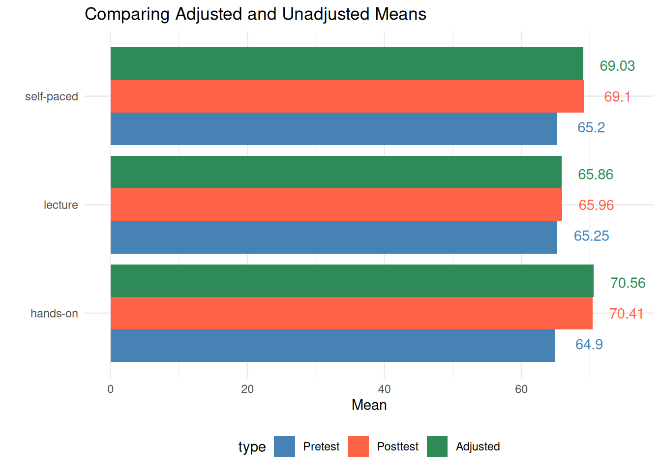
ANCOVA: Hypothesis Test IV
- [Example] Step #2
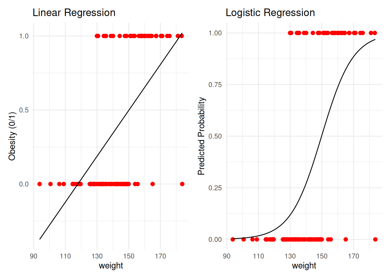
- What if we have a categorical outcome?
➤ Not related to this course, but categorical outcomes are commonly analyzed: - ✓ Examples: pass/fail a fitness test; pass/fail an academic test; retention (yes/no); on-time graduation (yes/no); proficiency (below, meeting, advanced), etc.
➔ These are not continuous, so we cannot use them in ANOVA
➤ Instead: logistic regression (PROC LOGISTIC or PROC GLM!) - ✓ Logistic regression can include both categorical and continuous IVs (and their interactions)
Code
# Load libraries
library(ggplot2)
library(dplyr)

# Simulate data
set.seed(123)
n <- 100
weight <- rnorm(n, 140, 20)
prob_obese <- 1 / (1 + exp(-(0.1 * weight -15)))  # logistic model
obese <- rbinom(n, size = 1, prob = prob_obese)

data <- data.frame(weight = weight, obese = obese)

# Linear model
lm_model <- lm(obese ~ weight, data = data)

# Logistic model
logit_model <- glm(obese ~ weight, data = data, family = "binomial")

# Prediction data
pred_data <- data.frame(weight = seq(min(weight), max(weight), length.out = 100))
pred_data$lm_pred <- predict(lm_model, newdata = pred_data)
pred_data$logit_pred <- predict(logit_model, newdata = pred_data, type = "response")

# Plot 1: Linear Regression
p1 <- ggplot(data, aes(x = weight, y = obese)) +
  geom_point(color = "red", size = 2) +
  geom_line(data = pred_data, aes(x = weight, y = lm_pred), color = "black") +
  labs(title = "Linear Regression", x = "weight", y = "Obesity (0/1)") +
  # ylim(0, 1.1) +
  theme_minimal()

# Plot 2: Logistic Regression
p2 <- ggplot(data, aes(x = weight, y = obese)) +
  geom_point(color = "red", size = 2) +
  geom_line(data = pred_data, aes(x = weight, y = logit_pred), color = "black") +
  labs(title = "Logistic Regression", x = "weight", y = "Predicted Probability") +
  # ylim(0, 1.1) +
  theme_minimal()

# Combine plots using patchwork
library(patchwork)
p1 + p2