To test one certain chunk of code, you click the “copy” icon in the upper right hand side of the chunk block (see screenshot below)
To review the whole file, click “</> Code” next to the title of this paper. Find “View Source” and click the button. Then, you can paste to the newly created Quarto Document.
2 R SYNTAX AND NAMING CONVENTIONS
Hide the code
# MAKE FRIENDS WITH R# BASED ON MAKE FRIENDS WITH R BY JONATHAN TEMPLIN# CREATED BY JIHONG ZHANG# R comments begin with a # -- there are no multiline comments# RStudio helps you build syntax# GREEN: Comments and character values in single or double quotes# You can use the tab key to complete object names, functions, and arugments# R is case sensitive. That means R and r are two different things.
3 R Functions
Hide the code
# In R, every statement is a function# The print function prints the contents of what is inside to the consoleprint(x =10)
[1] 10
Hide the code
# The terms inside the function are called the arguments; here print takes x# To find help with what the arguments are use:?print# Each function returns an objectprint(x =10)
[1] 10
Hide the code
# You can determine what type of object is returned by using the class functionclass(print(x =10))
[1] 10
[1] "numeric"
4 R Objects
Hide the code
# Each objects can be saved into the R environment (the workspace here)# You can save the results of a function call to a variable of any nameMyObject =print(x =10)
[1] 10
Hide the code
class(MyObject)
[1] "numeric"
Hide the code
# You can view the objects you have saved in the Environment tab in RStudio# Or type their nameMyObject
[1] 10
Hide the code
# There are literally thousands of types of objects in R (you can create them),# but for our course we will mostly be working with data frames (more later)# The process of saving the results of a function to a variable is called # assignment. There are several ways you can assign function results to # variables:# The equals sign takes the result from the right-hand side and assigns it to# the variable name on the left-hand side:MyObject =print(x =10)
[1] 10
Hide the code
# The <- (Alt "-" in RStudio) functions like the equals (right to left)MyObject2 <-print(x =10)
[1] 10
Hide the code
identical(MyObject, MyObject2)
[1] TRUE
Hide the code
# The -> assigns from left to right:print(x =10) -> MyObject3
[1] 10
Hide the code
identical(MyObject, MyObject2, MyObject3)
[1] TRUE
5 Importing and Exporting Data
The data frame is an R object that is a rectangular array of data. The variables in the data frame can be any class (e.g., numeric, character) and go across the columns. The observations are across the rows.
We will start by importing data from a comma-separated values (csv) file.
We will use the read.csv() function. Here, the argument stringsAsFactors keeps R from creating data strings
We will use here::here() function to quickly point to the target data file.
Hide the code
# Note: The argument file is the path to the file. If you opened this script directly in RStudio, then the current directory is the directory that contains the script. If the data file is in that directory, you can omit the full path. To find the current directory used in the environment, use the getwd() function.
getwd()
# Method 1: The most convientent way of importing data file is using the here packageroot_path <-getwd()HeightsData =read.csv(file = here::here(root_path, "data", "heights.csv"), stringsAsFactors =FALSE)head(HeightsData)
# If I tried to re-load the data, I would get an error:HeightsData =read.csv(file ="heights.csv", stringsAsFactors =FALSE)
Warning in file(file, "rt"): cannot open file 'heights.csv': No such file or
directory
Error in file(file, "rt"): cannot open the connection
Hide the code
# Method 2: I can use the full path to the file:HeightsData =read.csv(file ="/Users/jihong/Documents/website-jihong/posts/Lectures/2024-07-21-applied-multivariate-statistics-esrm64503/Lecture01/data/heights.csv", stringsAsFactors =FALSE)# Or, I can reset the current directory and use the previous syntax:setwd("/Users/jihong/Documents/website-jihong/posts/Lectures/2024-07-21-applied-multivariate-statistics-esrm64503/Lecture01/data/")HeightsData =read.csv(file ="heights.csv", stringsAsFactors =FALSE)HeightsData
# Note: Windows users will have to either change the direction of the slash# or put two slashes between folder levels.# To show my data in RStudio, I can either double click it in the # Environment tab or use the View() functionView(HeightsData)# You can see the variable names and contents by using the $:HeightsData$ID
[1] 1 2 3 4 5 6 7 8 9 10
Hide the code
# To read in SPSS files, we will need the foreign library. The foreign# library comes installed with R (so no need to use install.packages()).library(foreign)# The read.spss() function imports the SPSS file to an R data frame if the # argument to.data.frame is TRUEWideData =read.spss(file = here::here(root_path, "data", "wide.sav"), to.data.frame =TRUE)WideData
# The WideData and HeightsData have the same set of ID numbers. We can use the merge() function to merge them into a single data frame. Here, x is the name of the left-side data frame and y is the name of the right-side data frame. The arguments by.x and by.y are the name of the variable(s) by which we will merge:AllData =merge(x = WideData, y = HeightsData, by.x ="ID", by.y ="ID")AllData
         vars  n  mean   sd median trimmed  mad   min   max range  skew
ID          1 40  5.50 2.91   5.50    5.50 3.71  1.00 10.00  9.00  0.00
Gender      2 40  1.00 0.00   1.00    1.00 0.00  1.00  1.00  0.00   NaN
HeightIN    3 40 70.00 1.05  69.59   69.77 0.39 69.03 72.77  3.74  1.69
Time*       4 40  2.50 1.13   2.50    2.50 1.48  1.00  4.00  3.00  0.00
DV          5 40 22.27 2.12  22.50   22.31 2.22 16.50 26.50 10.00 -0.24
Age         6 40 11.14 2.25  11.25   11.14 2.89  7.90 14.40  6.50 -0.01
         kurtosis   se
ID          -1.31 0.46
Gender        NaN 0.00
HeightIN     1.92 0.17
Time*       -1.44 0.18
DV          -0.13 0.34
Age         -1.42 0.36
Hide the code
# We can use describeBy() to get descriptive statistics by groups:DescriptivesLongID =describeBy(AllDataLong, group = AllDataLong$ID)DescriptivesLongID
 Descriptive statistics by group
group: 1
         vars n  mean   sd median trimmed  mad   min   max range skew kurtosis
ID          1 4  1.00 0.00   1.00    1.00 0.00  1.00  1.00     0  NaN      NaN
Gender      2 4  1.00 0.00   1.00    1.00 0.00  1.00  1.00     0  NaN      NaN
HeightIN    3 4 72.77 0.00  72.77   72.77 0.00 72.77 72.77     0  NaN      NaN
Time        4 4  2.50 1.29   2.50    2.50 1.48  1.00  4.00     3 0.00    -2.08
DV          5 4 21.38 1.25  21.25   21.38 1.11 20.00 23.00     3 0.21    -1.92
Age         6 4 11.00 2.58  11.00   11.00 2.97  8.00 14.00     6 0.00    -2.08
           se
ID       0.00
Gender   0.00
HeightIN 0.00
Time     0.65
DV       0.62
Age      1.29
------------------------------------------------------------
group: 2
         vars n  mean   sd median trimmed  mad   min   max range skew kurtosis
ID          1 4  2.00 0.00   2.00    2.00 0.00  2.00  2.00   0.0  NaN      NaN
Gender      2 4  1.00 0.00   1.00    1.00 0.00  1.00  1.00   0.0  NaN      NaN
HeightIN    3 4 69.45 0.00  69.45   69.45 0.00 69.45 69.45   0.0  NaN      NaN
Time        4 4  2.50 1.29   2.50    2.50 1.48  1.00  4.00   3.0 0.00    -2.08
DV          5 4 23.00 2.12  22.75   23.00 2.22 21.00 25.50   4.5 0.14    -2.25
Age         6 4 11.12 2.62  11.10   11.12 2.97  8.10 14.20   6.1 0.02    -2.07
           se
ID       0.00
Gender   0.00
HeightIN 0.00
Time     0.65
DV       1.06
Age      1.31
------------------------------------------------------------
group: 3
         vars n  mean   sd median trimmed  mad  min  max range  skew kurtosis
ID          1 4  3.00 0.00   3.00    3.00 0.00  3.0  3.0   0.0   NaN      NaN
Gender      2 4  1.00 0.00   1.00    1.00 0.00  1.0  1.0   0.0   NaN      NaN
HeightIN    3 4 69.70 0.00  69.70   69.70 0.00 69.7 69.7   0.0   NaN      NaN
Time        4 4  2.50 1.29   2.50    2.50 1.48  1.0  4.0   3.0  0.00    -2.08
DV          5 4 23.75 2.33  24.25   23.75 1.48 20.5 26.0   5.5 -0.45    -1.83
Age         6 4 11.30 2.40  11.30   11.30 2.74  8.5 14.1   5.6  0.00    -2.07
           se
ID       0.00
Gender   0.00
HeightIN 0.00
Time     0.65
DV       1.16
Age      1.20
------------------------------------------------------------
group: 4
         vars n  mean   sd median trimmed  mad   min   max range skew kurtosis
ID          1 4  4.00 0.00   4.00    4.00 0.00  4.00  4.00   0.0  NaN      NaN
Gender      2 4  1.00 0.00   1.00    1.00 0.00  1.00  1.00   0.0  NaN      NaN
HeightIN    3 4 69.37 0.00  69.37   69.37 0.00 69.37 69.37   0.0  NaN      NaN
Time        4 4  2.50 1.29   2.50    2.50 1.48  1.00  4.00   3.0 0.00    -2.08
DV          5 4 24.88 1.25  24.75   24.88 1.11 23.50 26.50   3.0 0.21    -1.92
Age         6 4 11.55 2.45  11.55   11.55 2.82  8.70 14.40   5.7 0.00    -2.08
           se
ID       0.00
Gender   0.00
HeightIN 0.00
Time     0.65
DV       0.62
Age      1.23
------------------------------------------------------------
group: 5
         vars n  mean   sd median trimmed  mad   min   max range  skew kurtosis
ID          1 4  5.00 0.00   5.00    5.00 0.00  5.00  5.00     0   NaN      NaN
Gender      2 4  1.00 0.00   1.00    1.00 0.00  1.00  1.00     0   NaN      NaN
HeightIN    3 4 70.55 0.00  70.55   70.55 0.00 70.55 70.55     0   NaN      NaN
Time        4 4  2.50 1.29   2.50    2.50 1.48  1.00  4.00     3  0.00    -2.08
DV          5 4 22.62 0.85  22.75   22.62 0.74 21.50 23.50     2 -0.28    -1.96
Age         6 4 10.97 2.60  11.05   10.97 2.89  7.90 13.90     6 -0.05    -2.09
           se
ID       0.00
Gender   0.00
HeightIN 0.00
Time     0.65
DV       0.43
Age      1.30
------------------------------------------------------------
group: 6
         vars n  mean   sd median trimmed  mad   min   max range  skew kurtosis
ID          1 4  6.00 0.00   6.00    6.00 0.00  6.00  6.00   0.0   NaN      NaN
Gender      2 4  1.00 0.00   1.00    1.00 0.00  1.00  1.00   0.0   NaN      NaN
HeightIN    3 4 69.76 0.00  69.76   69.76 0.00 69.76 69.76   0.0   NaN      NaN
Time        4 4  2.50 1.29   2.50    2.50 1.48  1.00  4.00   3.0  0.00    -2.08
DV          5 4 21.12 1.03  21.00   21.12 0.74 20.00 22.50   2.5  0.27    -1.85
Age         6 4 10.93 2.49  10.95   10.93 2.82  8.00 13.80   5.8 -0.02    -2.07
           se
ID       0.00
Gender   0.00
HeightIN 0.00
Time     0.65
DV       0.52
Age      1.25
------------------------------------------------------------
group: 7
         vars n  mean   sd median trimmed  mad   min   max range skew kurtosis
ID          1 4  7.00 0.00   7.00    7.00 0.00  7.00  7.00   0.0  NaN      NaN
Gender      2 4  1.00 0.00   1.00    1.00 0.00  1.00  1.00   0.0  NaN      NaN
HeightIN    3 4 70.55 0.00  70.55   70.55 0.00 70.55 70.55   0.0  NaN      NaN
Time        4 4  2.50 1.29   2.50    2.50 1.48  1.00  4.00   3.0 0.00    -2.08
DV          5 4 23.00 1.47  22.75   23.00 1.11 21.50 25.00   3.5 0.35    -1.87
Age         6 4 11.12 2.52  11.10   11.12 2.82  8.20 14.10   5.9 0.02    -2.05
           se
ID       0.00
Gender   0.00
HeightIN 0.00
Time     0.65
DV       0.74
Age      1.26
------------------------------------------------------------
group: 8
         vars n  mean   sd median trimmed  mad   min   max range  skew kurtosis
ID          1 4  8.00 0.00   8.00    8.00 0.00  8.00  8.00   0.0   NaN      NaN
Gender      2 4  1.00 0.00   1.00    1.00 0.00  1.00  1.00   0.0   NaN      NaN
HeightIN    3 4 69.03 0.00  69.03   69.03 0.00 69.03 69.03   0.0   NaN      NaN
Time        4 4  2.50 1.29   2.50    2.50 1.48  1.00  4.00   3.0  0.00    -2.08
DV          5 4 23.38 0.48  23.25   23.38 0.37 23.00 24.00   1.0  0.32    -2.08
Age         6 4 10.97 2.65  11.00   10.97 3.04  7.90 14.00   6.1 -0.02    -2.10
           se
ID       0.00
Gender   0.00
HeightIN 0.00
Time     0.65
DV       0.24
Age      1.32
------------------------------------------------------------
group: 9
         vars n  mean   sd median trimmed  mad   min   max range  skew kurtosis
ID          1 4  9.00 0.00   9.00    9.00 0.00  9.00  9.00   0.0   NaN      NaN
Gender      2 4  1.00 0.00   1.00    1.00 0.00  1.00  1.00   0.0   NaN      NaN
HeightIN    3 4 69.49 0.00  69.49   69.49 0.00 69.49 69.49   0.0   NaN      NaN
Time        4 4  2.50 1.29   2.50    2.50 1.48  1.00  4.00   3.0  0.00    -2.08
DV          5 4 21.12 0.85  21.25   21.12 0.74 20.00 22.00   2.0 -0.28    -1.96
Age         6 4 11.20 2.74  11.25   11.20 3.11  8.00 14.30   6.3 -0.03    -2.11
           se
ID       0.00
Gender   0.00
HeightIN 0.00
Time     0.65
DV       0.43
Age      1.37
------------------------------------------------------------
group: 10
         vars n  mean   sd median trimmed  mad   min   max range  skew kurtosis
ID          1 4 10.00 0.00  10.00   10.00 0.00 10.00 10.00   0.0   NaN      NaN
Gender      2 4  1.00 0.00   1.00    1.00 0.00  1.00  1.00   0.0   NaN      NaN
HeightIN    3 4 69.29 0.00  69.29   69.29 0.00 69.29 69.29   0.0   NaN      NaN
Time        4 4  2.50 1.29   2.50    2.50 1.48  1.00  4.00   3.0  0.00    -2.08
DV          5 4 18.50 1.35  19.00   18.50 0.37 16.50 19.50   3.0 -0.68    -1.73
Age         6 4 11.20 2.53  11.15   11.20 2.82  8.30 14.20   5.9  0.04    -2.07
           se
ID       0.00
Gender   0.00
HeightIN 0.00
Time     0.65
DV       0.68
Age      1.27
9 Transforming Data
Hide the code
# Transforming data is accomplished by the creation of new variables. AllDataLong$AgeC = AllDataLong$Age -mean(AllDataLong$Age)# You can also use functions to create new variables. Here we create new terms# using the function for significant digits:AllDataLong$AgeYear =signif(x = AllDataLong$Age, digits =2)AllDataLong$AgeDecade =signif(x = AllDataLong$Age, digits =1)head(AllDataLong)
---title: "Lecture 01: Make Friends with R"format: html: toc: true toc_float: true toc_depth: 2 toc_collapsed: true number_sections: true code-fold: show code-summary: "Hide the code"---# How to use this file1. You can review all R code on this webpage.2. To test one certain chunk of code, you click the "copy" icon in the upper right hand side of the chunk block (see screenshot below) - 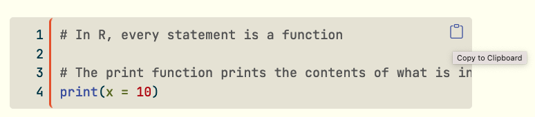3. To review the whole file, click "\</\> Code" next to the title of this paper. Find "View Source" and click the button. Then, you can paste to the newly created Quarto Document.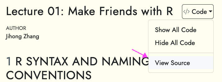# R SYNTAX AND NAMING CONVENTIONS```{r}#| eval: FALSE# MAKE FRIENDS WITH R# BASED ON MAKE FRIENDS WITH R BY JONATHAN TEMPLIN# CREATED BY JIHONG ZHANG# R comments begin with a # -- there are no multiline comments# RStudio helps you build syntax# GREEN: Comments and character values in single or double quotes# You can use the tab key to complete object names, functions, and arugments# R is case sensitive. That means R and r are two different things.```# R Functions```{r}# In R, every statement is a function# The print function prints the contents of what is inside to the consoleprint(x =10)# The terms inside the function are called the arguments; here print takes x# To find help with what the arguments are use:?print# Each function returns an objectprint(x =10)# You can determine what type of object is returned by using the class functionclass(print(x =10))```# R Objects```{r}# Each objects can be saved into the R environment (the workspace here)# You can save the results of a function call to a variable of any nameMyObject =print(x =10)class(MyObject)# You can view the objects you have saved in the Environment tab in RStudio# Or type their nameMyObject# There are literally thousands of types of objects in R (you can create them),# but for our course we will mostly be working with data frames (more later)# The process of saving the results of a function to a variable is called # assignment. There are several ways you can assign function results to # variables:# The equals sign takes the result from the right-hand side and assigns it to# the variable name on the left-hand side:MyObject =print(x =10)# The <- (Alt "-" in RStudio) functions like the equals (right to left)MyObject2 <-print(x =10)identical(MyObject, MyObject2)# The -> assigns from left to right:print(x =10) -> MyObject3identical(MyObject, MyObject2, MyObject3)```# Importing and Exporting Data- The data frame is an R object that is a rectangular array of data. The variables in the data frame can be any class (e.g., numeric, character) and go across the columns. The observations are across the rows.- We will start by importing data from a comma-separated values (csv) file.- We will use the read.csv() function. Here, the argument `stringsAsFactors` keeps R from creating data strings- We will use `here::here()` function to quickly point to the target data file.```{r}# Note: The argument file is the path to the file. If you opened this script directly in RStudio, then the current directory is the directory that contains the script. If the data file is in that directory, you can omit the full path. To find the current directory used in the environment, use the getwd() function. getwd()# To show the files in that directory, use the dir() function. You can see if the file you are opening is or is not in the current directory.dir()# Method 1: The most convientent way of importing data file is using the here packageroot_path <-getwd()HeightsData =read.csv(file = here::here(root_path, "data", "heights.csv"), stringsAsFactors =FALSE)head(HeightsData)``````{r}#| error: true# You can also set the directory using setwd(). Here, I set my directory to # my root folder:setwd("~")getwd()dir()# If I tried to re-load the data, I would get an error:HeightsData =read.csv(file ="heights.csv", stringsAsFactors =FALSE)``````{r}# Method 2: I can use the full path to the file:HeightsData =read.csv(file ="/Users/jihong/Documents/website-jihong/posts/Lectures/2024-07-21-applied-multivariate-statistics-esrm64503/Lecture01/data/heights.csv", stringsAsFactors =FALSE)# Or, I can reset the current directory and use the previous syntax:setwd("/Users/jihong/Documents/website-jihong/posts/Lectures/2024-07-21-applied-multivariate-statistics-esrm64503/Lecture01/data/")HeightsData =read.csv(file ="heights.csv", stringsAsFactors =FALSE)HeightsData``````{r}# Note: Windows users will have to either change the direction of the slash# or put two slashes between folder levels.# To show my data in RStudio, I can either double click it in the # Environment tab or use the View() functionView(HeightsData)# You can see the variable names and contents by using the $:HeightsData$ID# To read in SPSS files, we will need the foreign library. The foreign# library comes installed with R (so no need to use install.packages()).library(foreign)# The read.spss() function imports the SPSS file to an R data frame if the # argument to.data.frame is TRUEWideData =read.spss(file = here::here(root_path, "data", "wide.sav"), to.data.frame =TRUE)View(WideData) ```# Merging R data frame objects```{r}# The WideData and HeightsData have the same set of ID numbers. We can use the merge() function to merge them into a single data frame. Here, x is the name of the left-side data frame and y is the name of the right-side data frame. The arguments by.x and by.y are the name of the variable(s) by which we will merge:AllData =merge(x = WideData, y = HeightsData, by.x ="ID", by.y ="ID")AllData## Method 2: Use dplyr method, |> can be typed using `command + shift + M`library(dplyr)WideData |>left_join(HeightsData, by ="ID")```# Transforming Wide to Long```{r}# Sometimes, certain packages require repeated measures data to be in a long# format. library(dplyr) # contains variable selection ## Wrong WayAllData |> tidyr::pivot_longer(starts_with("DVTime"), names_to ="DV", values_to ="DV_Value") |> tidyr::pivot_longer(starts_with("AgeTime"), names_to ="Age", values_to ="Age_Value")## Correct WayAllData |> tidyr::pivot_longer(c(starts_with("DVTime"), starts_with("AgeTime"))) |> tidyr::separate(name, into =c("Variable", "Time"), sep ="Time") |> tidyr::pivot_wider(names_from ="Variable", values_from ="value") -> AllDataLong```# Gathering Descriptive Statistics```{r}# The psych package makes getting descriptive statistics very easy.## install.packages("psych")library(psych)# We can use describe() to get descriptive statistics across all cases:DescriptivesWide =describe(AllData)DescriptivesWideDescriptivesLong =describe(AllDataLong)DescriptivesLongView(AllDataLong)# We can use describeBy() to get descriptive statistics by groups:DescriptivesLongID =describeBy(AllDataLong, group = AllDataLong$ID)DescriptivesLongID#library(dplyr)AllDataLong |>group_by(ID) |>summarise(meanHeighID =mean(HeightIN),meanAge =mean(Age))```# Transforming Data```{r}# Transforming data is accomplished by the creation of new variables. AllDataLong$AgeC = AllDataLong$Age -mean(AllDataLong$Age)AllDataLong |>group_by(ID) |>mutate(StudentAvgAge =mean(Age)) |>mutate(AgeCbyStu = Age - StudentAvgAge) # You can also use functions to create new variables. Here we create new terms# using the function for significant digits:AllDataLong$AgeYear =signif(x = AllDataLong$Age, digits =2)AllDataLong$AgeYear =round(x = AllDataLong$AgeC, digits =2)View(AllDataLong)AllDataLong$AgeDecade =signif(x = AllDataLong$Age, digits =1)head(AllDataLong)AllDataLong |>mutate(AgeGroup =ifelse(Age <=12, 1, ifelse(Age <=14, 2, 3))) |>AllDataLong |>mutate(TimeNew =factor(Time, levels =1:4, labels =c("Pre", "Pre", "Post", "Post"))) ```

