Educational Statistics and Research Methods (ESRM) Program
University of Arkansas
Published
August 26, 2024
Learning Objectives
By the end of this lecture, you should be able to:
Load the ESRM64503 package and identify the variables in the lecture dataset.
Follow a data analysis plan to prepare and recode variables before analysis.
Describe marginal and joint distributions using numerical summaries and visualizations.
Explain and compute variance, covariance, and correlation, including the distinction between biased and unbiased variance estimators.
Specify and interpret general linear models that predict weight from height, gender, and their interaction.
Compare candidate models using residual variance, R^2, and nested-model tests.
Unit 1: Descriptive Statistics
Installation of ESRM64503 package
⌘+C
install.packages("devtools")devtools::install_github("JihongZ/ESRM64503") # Method 1pak::pak("JihongZ/ESRM64503") # Method 2: Install the Github packagepak::pak("JihongZ/ESRM64503", upgrade =TRUE) # If you already install the package, try to upgrade
Test ESTM64503 Package
package version
library(ESRM64503)devtools::package_info("ESRM64503") # Make sure the version number is 2024.08.20
 package   * version    date (UTC) lib source
 ESRM64503 * 2024.08.20 2026-08-31 [1] Github (JihongZ/ESRM64503@54cfc5b)

 [1] /Users/jihong/Rlibs
 [2] /Library/Frameworks/R.framework/Versions/4.4-arm64/Resources/library
 * ── Packages attached to the search path.
homework information
homework() # You can call "homework()" function to access homework info
There will be four homeworks in total for ESRM 64503.

Homework 0's answer:
Q2: In Rstudio, load the tidyverse package and copy-paste the console output of sessioninfo()
A2:
> sessionInfo()
R version 4.3.3 (2024-02-29)
Platform: aarch64-apple-darwin20 (64-bit)
Running under: macOS Sonoma 14.5

Matrix products: default
BLAS:   /System/Library/Frameworks/Accelerate.framework/Versions/A/Frameworks/vecLib.framework/Versions/A/libBLAS.dylib
LAPACK: /Library/Frameworks/R.framework/Versions/4.3-arm64/Resources/lib/libRlapack.dylib;  LAPACK version 3.11.0

locale:
[1] en_US.UTF-8/en_US.UTF-8/en_US.UTF-8/C/en_US.UTF-8/en_US.UTF-8

time zone: America/Chicago
tzcode source: internal

attached base packages:
[1] stats     graphics  grDevices utils     datasets  methods   base

other attached packages:
[1] cmdstanr_0.7.1     rstan_2.32.6       StanHeaders_2.32.9

loaded via a namespace (and not attached):
 [1] tensorA_0.36.2.1     utf8_1.2.4           generics_0.1.3       xml2_1.3.6           stringi_1.8.4
 [6] digest_0.6.37        magrittr_2.0.3       evaluate_0.24.0      grid_4.3.3           fastmap_1.2.0
[11] jsonlite_1.8.8       processx_3.8.4       pkgbuild_1.4.4       backports_1.5.0      ps_1.7.7
[16] gridExtra_2.3        fansi_1.0.6          viridisLite_0.4.2    QuickJSR_1.3.1       scales_1.3.0
[21] codetools_0.2-19     abind_1.4-5          cli_3.6.3            rlang_1.1.4          ESRM64503_2024.08.20
[26] munsell_0.5.1        tools_4.3.3          inline_0.3.19        parallel_4.3.3       checkmate_2.3.2
[31] dplyr_1.1.4          colorspace_2.1-1     ggplot2_3.5.1        kableExtra_1.4.0     curl_5.2.1
[36] vctrs_0.6.5          posterior_1.5.0      R6_2.5.1             matrixStats_1.3.0    stats4_4.3.3
[41] lifecycle_1.0.4      stringr_1.5.1        V8_5.0.0             pkgconfig_2.0.3      RcppParallel_5.1.9
[46] pillar_1.9.0         gtable_0.3.5         loo_2.7.0            glue_1.7.0           Rcpp_1.0.13
[51] systemfonts_1.1.0    xfun_0.47            tibble_3.2.1         tidyselect_1.2.1     rstudioapi_0.16.0
[56] knitr_1.48           htmltools_0.5.8.1    svglite_2.1.3        rmarkdown_2.28       compiler_4.3.3
[61] distributional_0.4.0

Q3: (Multiple-choice question) Assume you've already loaded the tidyverse and one dataset called flights in your R session, which R function below can get you know the number of rows AND columns of flights?
Note: you can load flights using the R code 'install.packages('nycflights13'); library(nycflights13)'
A3: Check all options.


You can work on HW1 now, please click the following link to have access:
https://jihongzhang.org/posts/Lectures/2024-07-21-applied-multivariate-statistics-esrm64503/HWs/HW_1.html
Data Files of ESRM64503
Data dataSexHeightWeight automate loaded
dataSexHeightWeight # You should find data named "dataSexHeightWeight" already loaded
   id sex heightIN weightLB
1   1   F       56      117
2   2   F       60      125
3   3   F       64      133
4   4   F       68      141
5   5   F       72      149
6   6   F       54      109
7   7   F       62      128
8   8   F       65      131
9   9   F       65      131
10 10   F       70      145
11 11   M       64      211
12 12   M       68      223
13 13   M       72      235
14 14   M       76      247
15 15   M       80      259
16 16   M       62      201
17 17   M       69      228
18 18   M       74      245
19 19   M       75      241
20 20   M       82      269
Type ? to check variable information of data
?dataSexHeightWeight
Simulated Data for Today’s Lecture - dataSexHeightWeight
To help demonstrate the concepts of today’s lecture, we will be using a toy data set with three variables
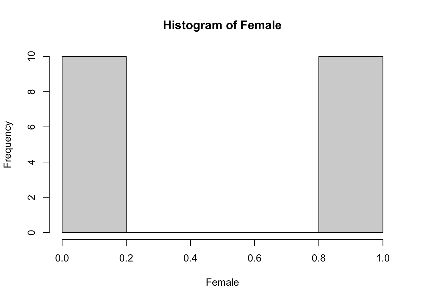
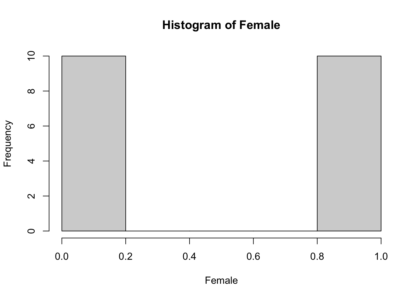
Female (Gender): Coded as Male (= 0) or Female (= 1)
In R, factor variable with two levels: FALSE, TRUE
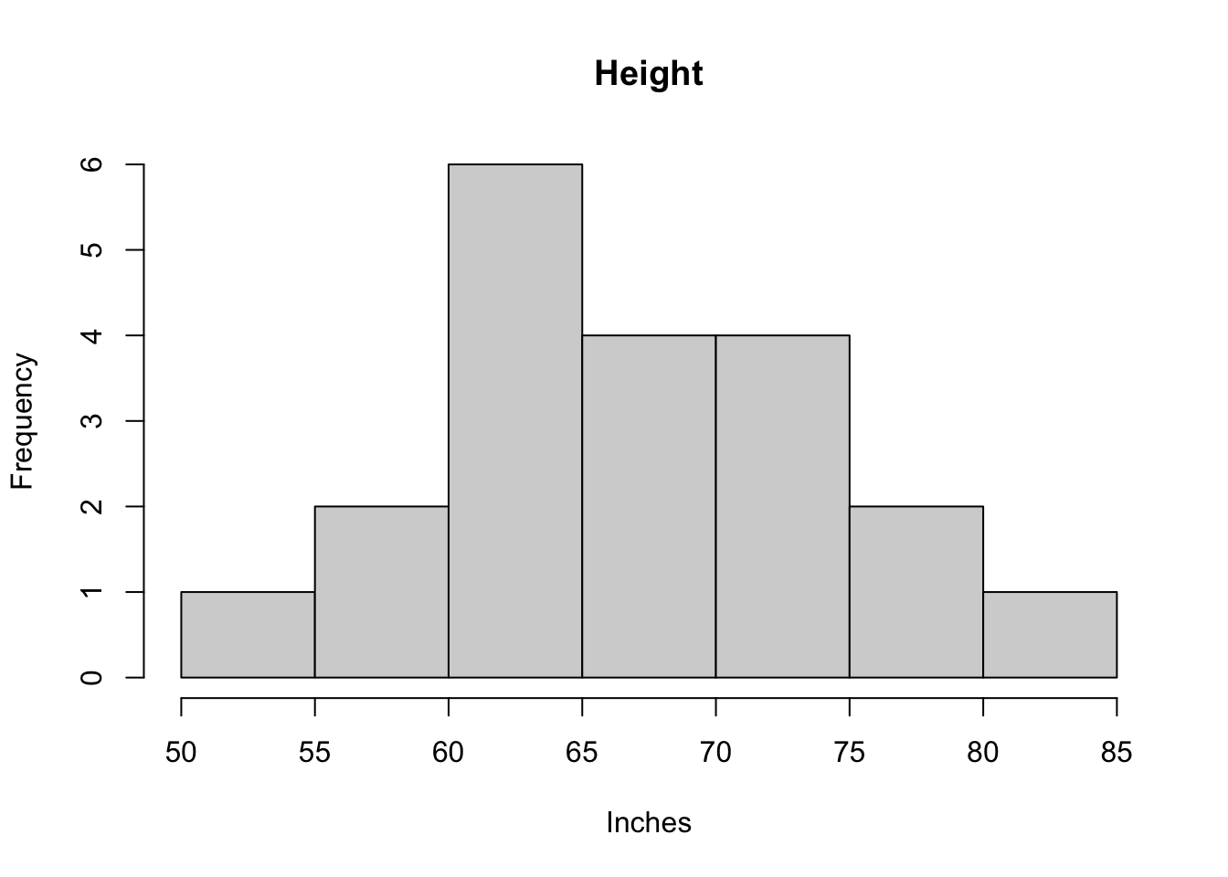
Height: in inches
Weight: in pounds
The goal of lecture 02 will be to build a general linear model that predicts a person’s weight
Linear (regression) model: a statistical model for an outcome that uses a linear combination (a weighted sum) of one or more predictor variables to produce an estimate of an observation’s predicted value
\mathbb{y} = \beta_0+\beta_1 \mathbf{X}
All models we learnt today will follow this framework.
Data Analysis Plan
Research question: How well do height and gender predict weight in this toy dataset?
Stage
What we will do
Purpose
1. Prepare
Check the sample and recode sex as female
Make the variables ready for analysis
2. Describe
Summarize height, weight, and gender
Understand each variable’s distribution
3. Relate
Examine scatterplots, correlations, and covariances
Describe how the variables vary together
4. Model
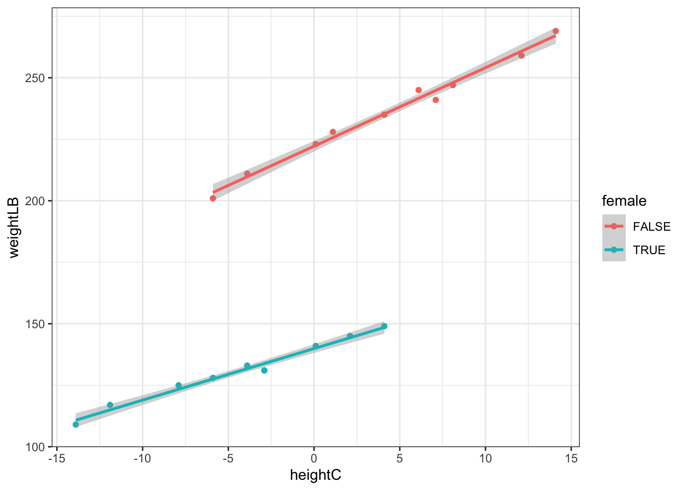
Predict weight from height, gender, and their interaction
Estimate each predictor’s contribution
5. Compare
Compare model fit and interpret the coefficients
Select and explain the most useful model
Workflow: Data preparation \rightarrow descriptive evidence \rightarrow candidate models \rightarrow model comparison and interpretation
Recode Variables
library(ESRM64503) # INSTALL: pak::pak("JihongZ/ESRM64504")library(kableExtra) # INSTALL: pak::pak("JihongZ/ESRM64504")## First checking sample size## N = 20## Recode Sex as FemaledataSexHeightWeight$female = dataSexHeightWeight$sex =="F"dataSexHeightWeight
toy data set
id
sex
heightIN
weightLB
female
1
F
56
117
TRUE
2
F
60
125
TRUE
3
F
64
133
TRUE
4
F
68
141
TRUE
5
F
72
149
TRUE
6
F
54
109
TRUE
7
F
62
128
TRUE
8
F
65
131
TRUE
9
F
65
131
TRUE
10
F
70
145
TRUE
11
M
64
211
FALSE
12
M
68
223
FALSE
13
M
72
235
FALSE
14
M
76
247
FALSE
15
M
80
259
FALSE
16
M
62
201
FALSE
17
M
69
228
FALSE
18
M
74
245
FALSE
19
M
75
241
FALSE
20
M
82
269
FALSE
Descriptive Statistics
First, we can inspect each variable individually (marginal distribution) through a set of descriptive statistics
Visual way: histogram plot or density plot
Statistical way: Central tendency and Variability
Mean, Median, Mode
SD, Range
Second, we can also summarize the joint (bivariate) distribution of two variables through a set of descriptive statistics:
Joint vs. Marginal: joint distribution describes more than one variable simultaneously
Common bivariate descriptive statistics:
Correlation and covariance
Quick inspection: Missing data rate
Check (1) if any case has missing value (2) distributions for continuous and categorical variables
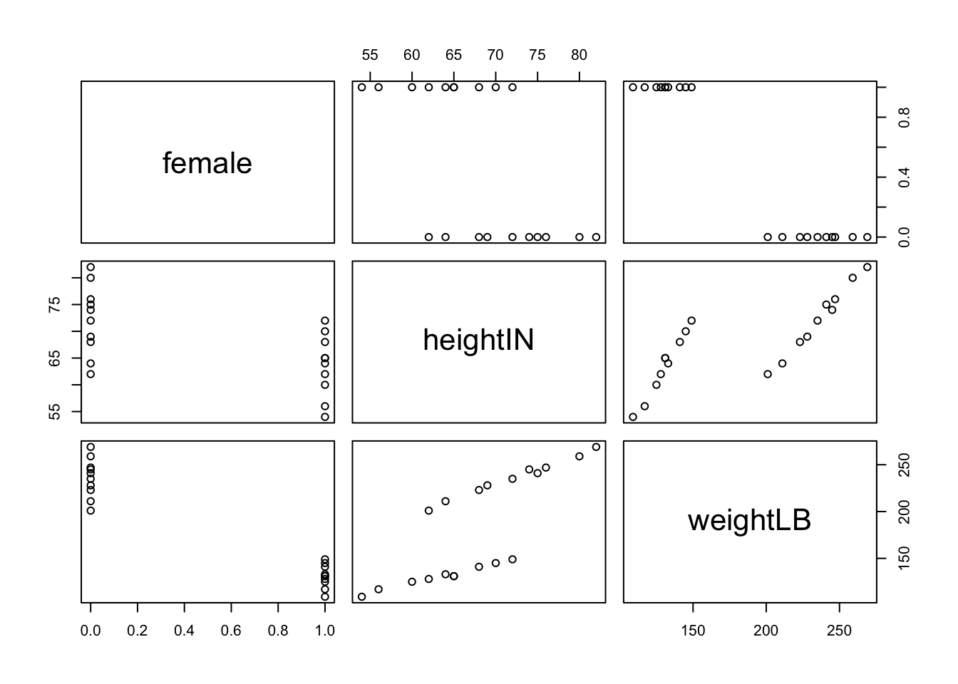
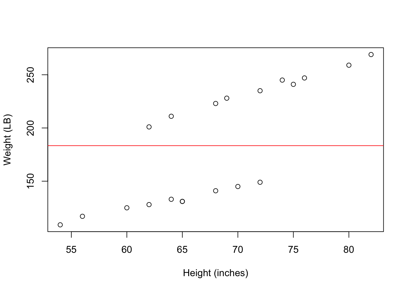
Question: What conclusions we can draw regarding the relationships among three variables?
variables <-c("heightIN", "weightLB", "female")analysis_data <- dataSexHeightWeight[, variables]covariance_matrix <-cov(analysis_data)correlation_matrix <-cor(analysis_data)# The covariance matrix already has variances on its diagonalcor_cov_mat <- covariance_matrix# Replace its lower half with the corresponding correlationslower_half <-lower.tri(cor_cov_mat)cor_cov_mat[lower_half] <- correlation_matrix[lower_half]cor_cov_mat
heightIN
weightLB
female
heightIN
55.358
334.832
-2.263
weightLB
0.798
3179.095
-27.632
female
-0.593
-0.955
0.263
Variance, Correlation, Covariance
Re-examining the Concept of Variance
Variability is a central concept in advanced statistics
In multivariate statistic, covariance is also central
Two formulas for the variance (about the same when N is larger):
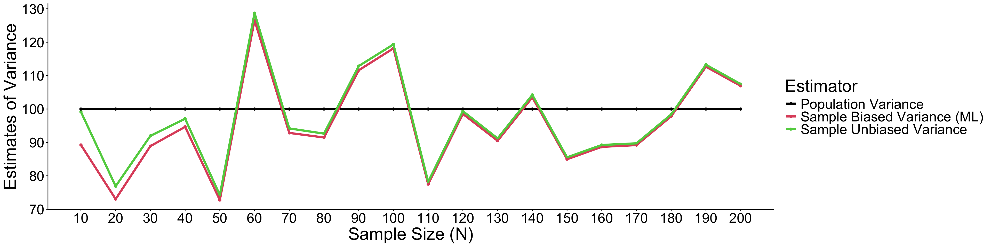
Take home note: Unbiased variance estimators can get more accurate estimate of variance than the biased one.
Biased VS. Unbiased Estimator of Variance (Cont.)
⌘+C
library(ggplot2)variance_mat |>as.data.frame() |>pivot_longer(-sample_size) |>ggplot() +geom_point(aes(x = sample_size, y = value, color = name), linewidth =1.1) +geom_line(aes(x = sample_size, y = value, color = name), linewidth =1.5) +labs(x ="Sample Size (N)", y ="Estimates of Variance") +scale_color_manual(values =1:3, labels =c("Population Variance", "Sample Biased Variance (ML)", "Sample Unbiased Variance"), name ="Estimator") +scale_x_continuous(breaks =seq(10, 200, 10)) +theme_classic() +theme(text =element_text(size =25))
Take home note: When sample size is small, unbiased variance estimators can get the estimate of variance closer to the population variance than the biased one.
Interpretation of Variance
The variance (\sigma^2 and S^2) describes the spread of a variable in squared units (which come from (Y_p - \bar Y)^2 term in the equation)
Variance: the average squared distance of an observation from the mean
For the toy sample, the variance of height is 55.358 inches squared
For the toy sample, the variance of weight is 3179.095 pounds squared
The variance of female — not applicable in the same way!
How is the sample equally distributed across different groups: 50/50 -> largest variance
Because squared units are difficult to work with, we typically use the standard deviation – which is reported in units
Standard deviation: the average distance of an observation from the mean
SD of Height: 7.44 inches
SD of Weight: 56.383 pounds
Variance/SD as a More General Statistical Concept
Variance (and the standard deviation) is a concept that is applied across statistics – not just for data
Statistical parameters (slope, intercept) have variance
e.g., The sample mean \bar Y has a “standard error” (SE) of S_{\bar Y} = S_Y / \sqrt{N}
How accurately we can estimate the sample mean \neq How dispersed the samples are
The standard error is another name for standard deviation
So “standard error of the mean” is equivalent to “standard deviation of the mean”
Usually “error” refers to parameters; “deviation” refers to data
Variance of the mean would be S_{\bar Y}^2 = S^2_Y / N
Example: Table of Descriptive Statistics
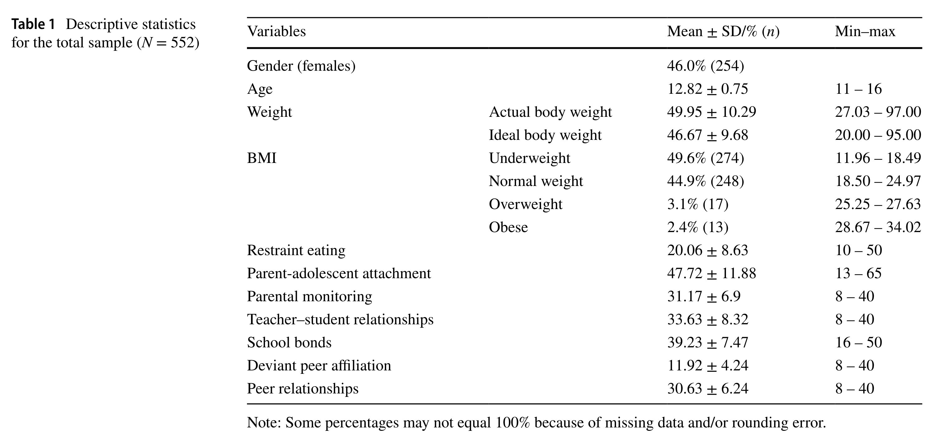
Table 1 (Xiong et al., 2023)
Key information that be reprted
All variables that you think relevant to the study: (1) demographic (2) context factors (3) outcomes or predictors
Categorical Variables: (1) Percentage of each level (2) Sample size of each level (3) Range
Continuous Variables: Mean + SD + Range
Correlation of Variables
Moving from marginal summaries of each variable to joint (bivariate) summaries, we can use the Pearson Correlation to describe the association between a pair of continuous variables:
Alternatively, we cab describe the relationships between two or more variables using their joint distributions
Visual way: Scatter plot, Group-level Histogram
Statistical way: Covariance, Pearson Correlation, Chi-square (\chi^2) test
Unit 2: General Linear Model
Learning Objectives
Types of distributions:
Conditional distribution: a special joint distribution condition on other variable
The General Linear Model
Regression
Analysis of Variance (ANOVA)
Analysis of Covariance (ANCOVA)
Beyond – Interactions
Taxonomy of GLM
The general linear model (GLM) incorporates many different labels of analysis under one unifying umbrella:
Categorical Xs
Continuous Xs
Both Types of Xs
Univariate Y
ANOVA
Regression
ANCOVA
Multivariate Ys
MANOVA
Multivariate Regression
MANCOVA
The typical assumption is that error term (residual or \epsilon) is normally distribution – meaning that the data are conditionally normally distributed
Models for non-normal outcomes (e.g., dichotomous, categorical, count) fall under the Generalized Linear Model, of which general linear model is a special case
Note: because gender is a categorical predictor, we must first code it into a number before entering it into model (typically done automatically in software)
Here we code the variable as Female = 1 for females; Female = 0 for males
Estimated parameters:
\beta_0: Intercept - predicted value of Weight for a person with Female = 0 (males)
\beta_2: Slope of Female - Change in predicted value of Weight between Males and Famales
R Code
model3 <-lm(weightLB ~ female, data = dataSexHeightWeight) # model formulasummary(model3)$coefficients # regression cofficients table
            Estimate Std. Error   t value     Pr(>|t|)
(Intercept)    235.9   5.414897  43.56500 1.062177e-19
femaleTRUE    -105.0   7.657821 -13.71147 5.736338e-11
anova(model3) # F-statistic table
Analysis of Variance Table

Response: weightLB
          Df Sum Sq Mean Sq F value    Pr(>F)
female     1  55125   55125     188 5.736e-11 ***
Residuals 18   5278     293
---
Signif. codes:  0 '***' 0.001 '**' 0.01 '*' 0.05 '.' 0.1 ' ' 1
Interpretation
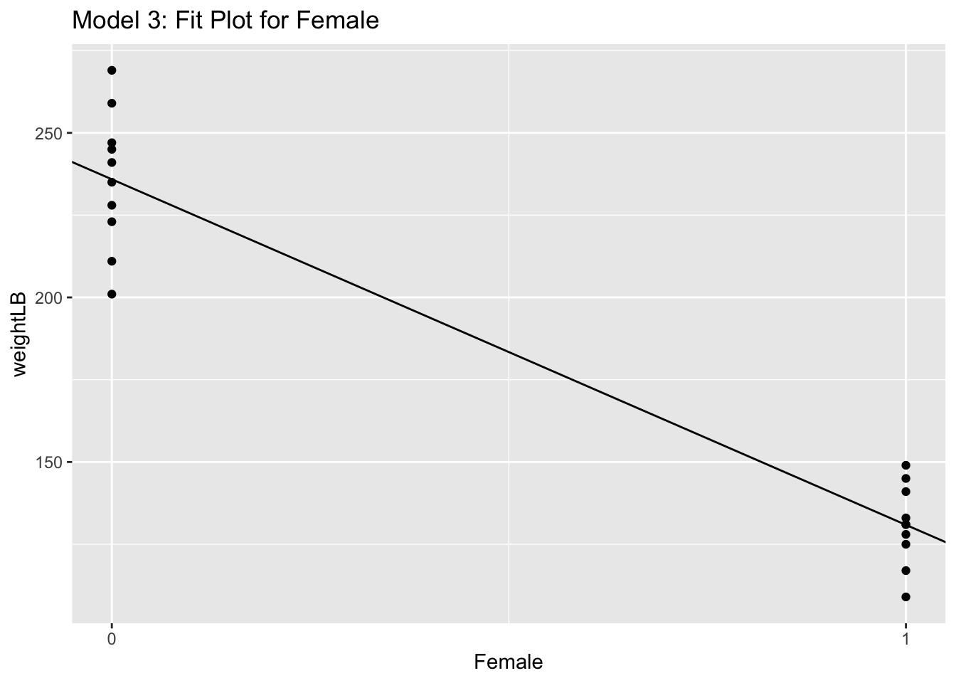
\beta_0 = 235.9 pounds is the predicted value of a Weight for a male
\beta_0 +\beta_1 = 235.9 - 105.0 = 130.9 pounds is the predicted value of a Weight for a female
\beta_1 = 105 expected difference between gender, which is significant based on t-test and F-test
Visualization:
Line Plot (not frequently used in this case)
ggplot(dataSexHeightWeight) +geom_point(aes(x =as.numeric(female), y = weightLB)) +geom_abline(intercept =coef(model3)[1], slope =coef(model3)[2]) +scale_x_continuous(breaks =0:1) +labs(title ="Model 3: Fit Plot for Female",x ="Female")
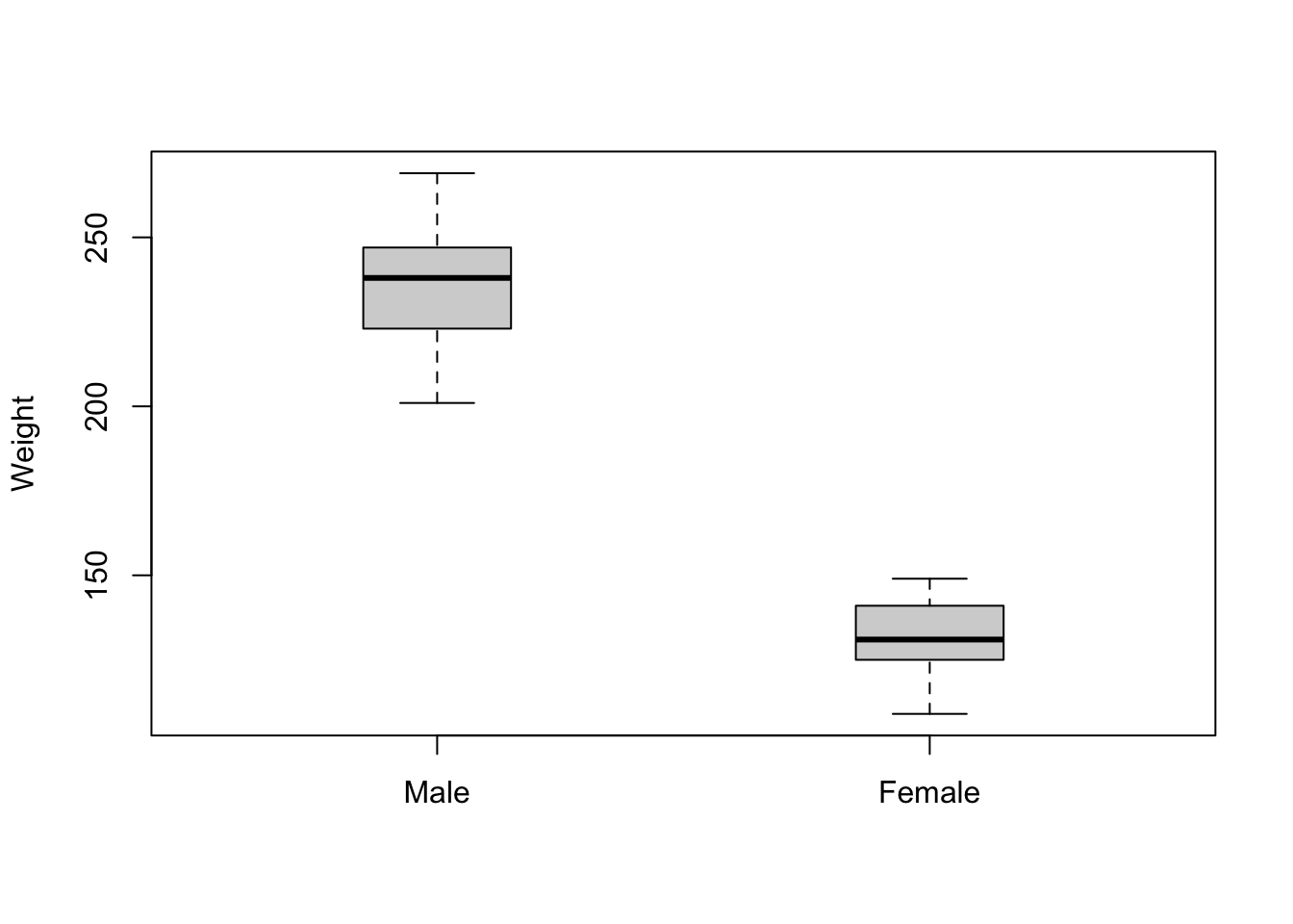
Visualization: box-and-whisker plot (Basic Way)
boxplot(weightLB ~ female, data = dataSexHeightWeight, names =c("Male", "Female"), ylab ="Weight", xlab ="",boxwex = .3) # Basic boxplot in R
Visualization: box-and-whisker plot (Fancy Way)
ggplot2 package
ggplot(dataSexHeightWeight, aes(x = female, y = weightLB)) +geom_dotplot(aes(fill = female, color = female), binaxis='y', stackdir='center') +stat_summary(fun.data="mean_cl_normal", fun.args =list(conf.int=.75), geom="crossbar", width=0.3, fill ="yellow", alpha = .5) +stat_summary(fun.data="median_hilow", geom="errorbar", fun.args =list(conf.int=1), width = .1, color="black") +# Mean +- 2SD stat_summary(fun.data="mean_sdl", geom="point", shape =5, size =3) +scale_x_discrete(labels =c("Male", "Female")) +labs(x ="", y ="Weight") +theme_bw() +theme(legend.position ="none", text =element_text(size =20))
Total explained variances in weight by height and gender: Multiple R^2 of Model 5
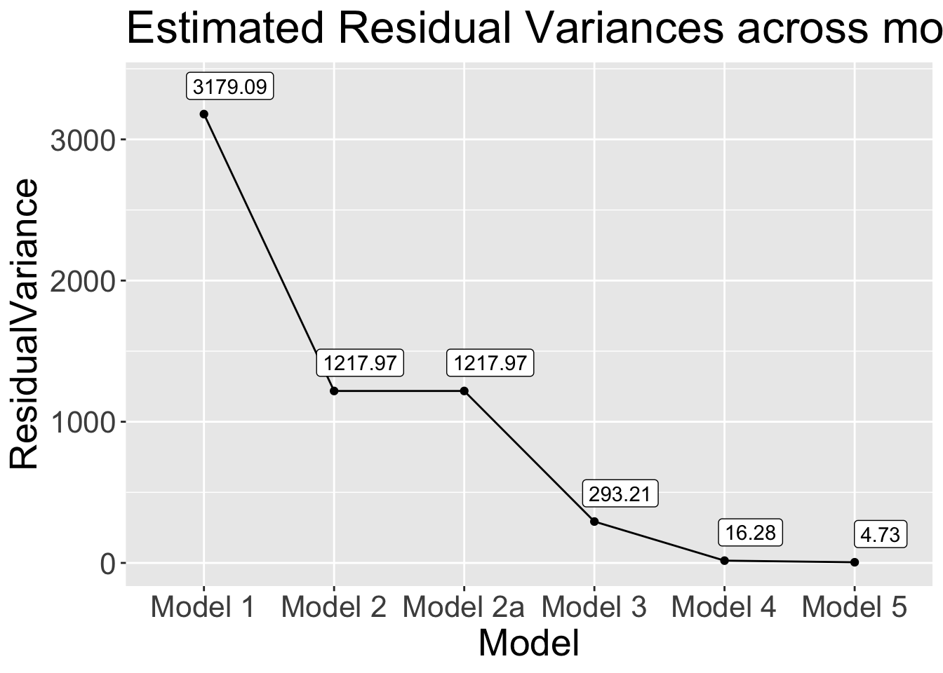
(3179.09-4.73)/3179.09 = 0.9985\rightarrow 99.85% variances in weights can be explained by height and gender
F-test comparing Model 5 to Model 1
F_{3, 16} = 4250.1, p < .001
⌘+C
summary(model5)
Call:
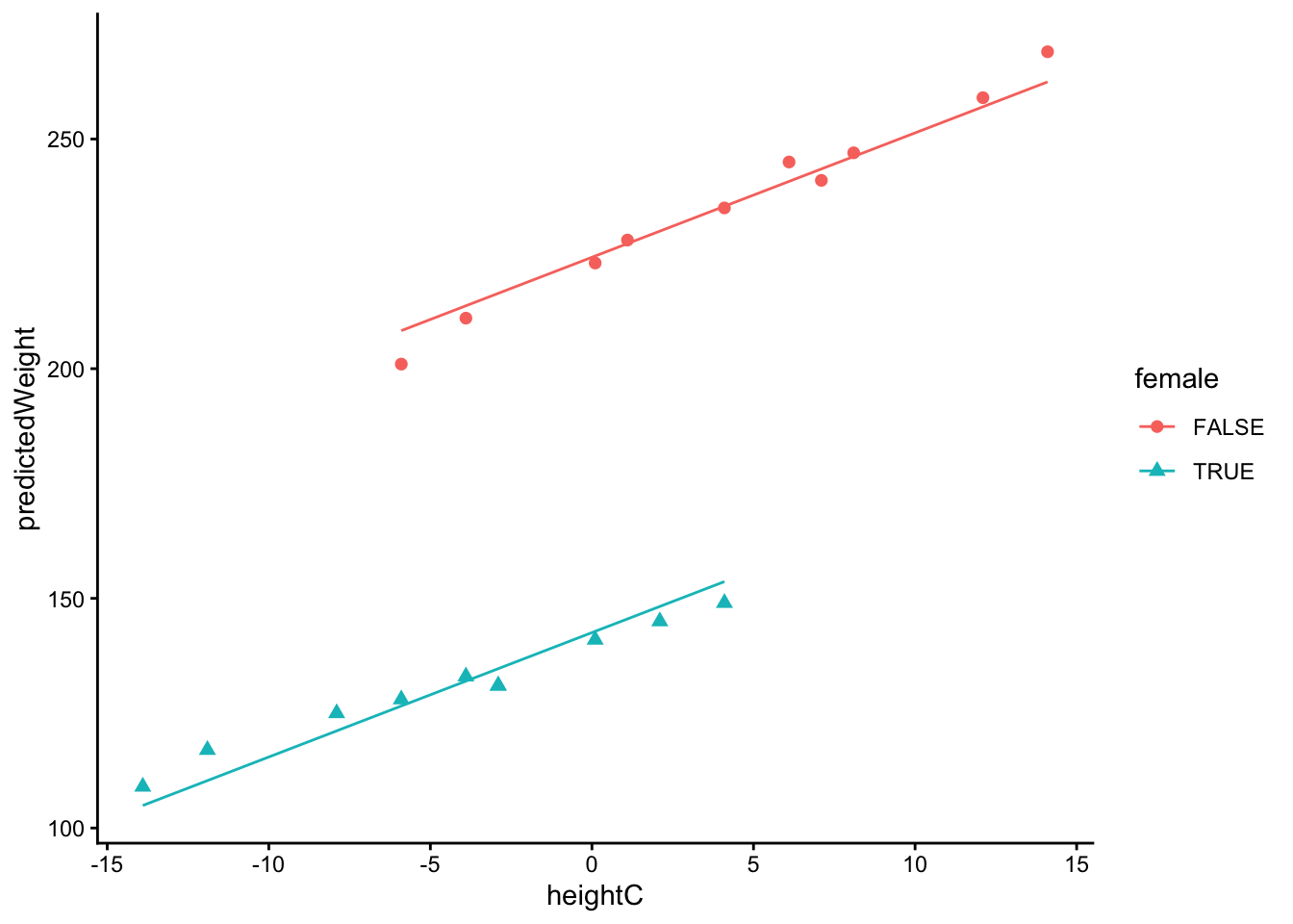
lm(formula = weightLB ~ heightC * female, data = dataSexHeightWeight)

Residuals:
    Min      1Q  Median      3Q     Max
-3.8312 -1.7797  0.4958  1.3575  3.3585

Coefficients:
                   Estimate Std. Error t value Pr(>|t|)
(Intercept)        222.1842     0.8381  265.11  < 2e-16 ***
heightC              3.1897     0.1114   28.65 3.55e-15 ***
femaleTRUE         -82.2719     1.2111  -67.93  < 2e-16 ***
heightC:femaleTRUE  -1.0939     0.1678   -6.52 7.07e-06 ***
---
Signif. codes:  0 '***' 0.001 '**' 0.01 '*' 0.05 '.' 0.1 ' ' 1

Residual standard error: 2.175 on 16 degrees of freedom
Multiple R-squared:  0.9987,    Adjusted R-squared:  0.9985
F-statistic:  4250 on 3 and 16 DF,  p-value: < 2.2e-16
Are Height alone a good predictor?
Explained remaining variances in weight by height: Multiple R^2 of Model 5 to Model 3
(293.21-4.73)/293.21 = 0.9839\rightarrow 98.39% variances in weights remaining after gender can be explained by the main and interaction effects of height
F-test comparing Model 5 to Model 3
F_{2, 16} = 548.74, p < .001 suggests the effect of hight on weight is significant after controlling the effect of gender
True explained variances out of total variances in weight: Unique contribution of adding Height into the model
Check model 3, we can found that gender explained 90.78% variance of weight
0.9839 * (1 - 0.9078) = 0.0907\rightarrow 9.07% more variances of weights can be explained by height after gender is already in the model
90.78% + 9.07% = 99.85% is the total variance explained by height and gender
Are gender alone a good predictor?
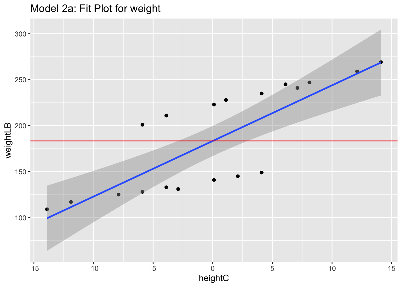
Explained remaining variances in weight by gender: Multiple R^2 of Model 5 to Model 2a
(1217.97-4.73)/1217.97 = 0.9961\rightarrow 99.61% variances in weights remaining after height can be explained by the main and interaction effects of gender
F-test comparing Model 5 to Model 2a
F_{2, 16} = 2308.8, p < .001 suggests the effect of gender on weight is significant after controlling the effect of height