install.packages("lavaan")Outline
Today's Class
- Multivariate linear models: An introduction
- How to form multivariate models in lavaan
- What parameters mean
- How they relate to the multivariate normal distribution
Multivariate Models: An Introduction
Multivariate Linear Models
- The next set of lectures is provided to give an overview of multivariate linear models
- Models for more than one dependent/outcome variables
- Our focus today will be on models where the DV is plausibly continuous
- so we’ll use error terms that are multivariate-normally distributed
- Not a necessity – generalized multivariate models are possible
Classical vs. Contemporary Methods
In “classical” multivariate textbooks and classes, multivariate linear models fall under the names of Multivariate ANOVA (MANOVA) and multivariate regression
These methods rely upon least squares estimation, which:
- Inadequate with missing data
- Offers very limited methods of setting covariance matrix structures
- Does not allow for different sets of predictor variables for each outcome
- Does not give much information about model fit
- Does not provide adequate model comparison procedures
The classical methods have been subsumed into the modern (likelihood- or Bayes-based) multivariate methods
- Subsume: include or absorb (something) in something else
- Meaning: modern methods do what classical methods do (and more)
Contemporary Methods for Estimating Multivariate Linear Models
We will discuss three large classes of multivariate linear modeling methods:
- Path analysis models (typically through structural equation modeling and path analysis software)
- Linear mixed models (typically through linear models software)
- Psychological network models (typically through psychological network software)
- Bayesian networks (frequently not mentioned in the social sciences but subsume all we are doing)
The theory behind each is identical—the main difference is software
Some software does a lot (
Mplussoftware is likely the most complete), but none (as of 2024) does it allWe will start with path analysis (via the
lavaanpackage) as the modeling method is more direct, and then move to linear mixed-models software (via thenlmeandlme4packages)Bayesian networks will be discussed in the Bayes section of the course and will use entirely different software
Biggest Difference From Univariate Models: Model Fit
- In univariate linear models, the “model for the variance” wasn’t much of a model; there was one variance term possible (\sigma^2_e) and one term estimated
- A saturated model: all variances/covariances are freely estimated without any constraints—model fit was always perfect
- For example, a correlation matrix of 3 variables can be estimated upto 3 parameters.
- In multivariate linear models, because of the number of variances/covariances, oftentimes models are not saturated for the variances
- Therefore, model fit becomes an issue
- Any non-saturated model for the variances must be shown to fit the data before being used for interpretation
- “Fit the data” has differing standards depending on the software used.
Today’s Example Data
Data are simulated based on the results reported in:
Sample of 350 undergraduates (229 women, 121 men)
- In simulation, 10% of variables were missing (using missing completely at random mechanism).
Make sure you install
lavaanpackage
TipDictionary
- Prior Experience at High School Level (HSL)
- Prior Experience at College Level (CC)
- Perceived Usefulness of Mathematics (USE)
- Math Self-Concept (MSC)
- Math Anxiety (MAS)
- Math Self-Efficacy (MSE)
- Math Performance (PERF)
- Female (sex variable: 0 = male; 1 = female)
⌘+C
library(ESRM64503)
library(kableExtra)
library(tidyverse)
library(DescTools) # Desc() allows you to quick screen data
options(digits=3)
head(dataMath) id hsl cc use msc mas mse perf female
1 1 NA 9 44 55 39 NA 14 1
2 2 3 2 77 70 42 71 12 0
3 3 NA 12 64 52 31 NA NA 1
4 4 6 20 71 65 39 84 19 0
5 5 2 15 48 19 2 60 12 0
6 6 NA 15 61 62 42 87 18 0Desc() in package DescTools allows you to quick screen data
dim(dataMath)
Desc(dataMath[,2:8], plotit = FALSE, conf.level = FALSE)[1] 350 9
──────────────────────────────────────────────────────────────────────────────
Describe dataMath[, 2:8] (data.frame):
data frame: 350 obs. of 7 variables
145 complete cases (41.4%)
Nr Class ColName NAs Levels
1 int hsl 36 (10.3%)
2 int cc 37 (10.6%)
3 int use 24 (6.9%)
4 int msc 39 (11.1%)
5 int mas 46 (13.1%)
6 int mse 34 (9.7%)
7 int perf 60 (17.1%)
──────────────────────────────────────────────────────────────────────────────
1 - hsl (integer)
length n NAs unique 0s mean meanCI'
350 314 36 8 0 4.92 4.92
89.7% 10.3% 0.0% 4.92
.05 .10 .25 median .75 .90 .95
3.00 3.00 4.00 5.00 6.00 6.00 7.00
range sd vcoef mad IQR skew kurt
7.00 1.32 0.27 1.48 2.00 -0.26 -0.41
value freq perc cumfreq cumperc
1 1 1 0.3% 1 0.3%
2 2 11 3.5% 12 3.8%
3 3 34 10.8% 46 14.6%
4 4 71 22.6% 117 37.3%
5 5 79 25.2% 196 62.4%
6 6 88 28.0% 284 90.4%
7 7 27 8.6% 311 99.0%
8 8 3 1.0% 314 100.0%
' 0%-CI (classic)
──────────────────────────────────────────────────────────────────────────────
2 - cc (integer)
length n NAs unique 0s mean meanCI'
350 313 37 28 21 10.31 10.31
89.4% 10.6% 6.0% 10.31
.05 .10 .25 median .75 .90 .95
0.00 2.00 6.00 10.00 14.00 19.00 20.00
range sd vcoef mad IQR skew kurt
27.00 5.89 0.57 5.93 8.00 0.17 -0.43
lowest : 0 (21), 1 (5), 2 (9), 3 (9), 4 (12)
highest: 23, 24, 25, 26, 27
heap(?): remarkable frequency (8.6%) for the mode(s) (= 10, 13)
' 0%-CI (classic)
──────────────────────────────────────────────────────────────────────────────
3 - use (integer)
length n NAs unique 0s mean meanCI'
350 326 24 71 1 52.50 52.50
93.1% 6.9% 0.3% 52.50
.05 .10 .25 median .75 .90 .95
25.50 31.00 42.25 52.00 64.00 71.50 77.75
range sd vcoef mad IQR skew kurt
100.00 15.81 0.30 16.31 21.75 -0.11 -0.08
lowest : 0, 13, 15, 16, 19 (2)
highest: 84 (2), 86, 92, 95, 100
' 0%-CI (classic)
──────────────────────────────────────────────────────────────────────────────
4 - msc (integer)
length n NAs unique 0s mean meanCI'
350 311 39 76 0 49.79 49.79
88.9% 11.1% 0.0% 49.79
.05 .10 .25 median .75 .90 .95
24.00 29.00 38.00 49.00 61.00 72.00 80.50
range sd vcoef mad IQR skew kurt
98.00 16.96 0.34 16.31 23.00 0.23 -0.09
lowest : 5, 9, 12, 15, 16 (2)
highest: 87 (3), 89, 91, 94, 103
' 0%-CI (classic)
──────────────────────────────────────────────────────────────────────────────
5 - mas (integer)
length n NAs unique 0s mean meanCI'
350 304 46 57 1 31.50 31.50
86.9% 13.1% 0.3% 31.50
.05 .10 .25 median .75 .90 .95
13.00 17.00 24.75 32.00 39.00 45.70 50.00
range sd vcoef mad IQR skew kurt
62.00 11.32 0.36 10.38 14.25 -0.13 -0.17
lowest : 0, 2, 3 (2), 5, 6
highest: 54 (2), 55 (2), 56, 58, 62
' 0%-CI (classic)
──────────────────────────────────────────────────────────────────────────────
6 - mse (integer)
length n NAs unique 0s mean meanCI'
350 316 34 56 0 73.41 73.41
90.3% 9.7% 0.0% 73.41
.05 .10 .25 median .75 .90 .95
54.00 58.00 65.00 73.00 81.00 88.50 92.25
range sd vcoef mad IQR skew kurt
60.00 11.89 0.16 11.86 16.00 0.06 -0.26
lowest : 45 (2), 46, 47, 49 (2), 50 (4)
highest: 98, 100, 101 (2), 103, 105 (2)
' 0%-CI (classic)
──────────────────────────────────────────────────────────────────────────────
7 - perf (integer)
length n NAs unique 0s mean meanCI'
350 290 60 19 0 13.97 13.97
82.9% 17.1% 0.0% 13.97
.05 .10 .25 median .75 .90 .95
9.45 10.00 12.00 14.00 16.00 18.00 19.00
range sd vcoef mad IQR skew kurt
18.00 2.96 0.21 2.97 4.00 0.16 0.14
lowest : 5, 6, 7 (2), 8 (3), 9 (8)
highest: 19 (10), 20 (4), 21 (3), 22 (2), 23
heap(?): remarkable frequency (13.8%) for the mode(s) (= 13)
' 0%-CI (classic)Using MVN Likelihoods in lavaan
The lavaan package is developed by Dr. Yves Rosseel to provide useRs, researchers and teachers a free open-source, but commercial-quality package for latent variable modeling. You can use lavaan to estimate a large variety of multivariate statistical models, including path analysis, confirmatory factor analysis, structural equation modeling and growth curve models.
lavaan’s default model is a linear (mixed) model that uses ML with the multivariate normal distributionML is sometimes called a full-information method (FIML)
- Full information is the term used when each observation is used in a likelihood function
The contrast is limited information (not all observations are used; typically summary statistics are used)
install.packages('lavaan')
library(lavaan)Revisiting Univariate Linear Regression
- We will begin our discussion with perhaps the simplest model we will see: a univariate empty model
- We will use the PERF variable from our example data: Performance on a mathematics assessment
- The empty model for PERF is:
- e_{i, PERF} \sim N(0, \sigma^2_{e,PERF})
- Two parameters are estimated: \beta_{0,PERF} and \sigma^2_{e,PERF}
\text{PERF}_i = \beta_{0,\color{tomato}{PERF}} + e_{i, \color{tomato}{PERF}}
- Here, the additional subscript is added to denote these terms are part of the model for the PERF variable
- We will need these when we get to multivariate models and path analysis
lavaan Syntax: General
- Estimating a multivariate model using
lavaancontains three steps:- Model building: Build a string object including syntax for models (e.g.,
model01.syntax) - Model fitting: Estimate the model with observed data and save it to a fit object (e.g.,
model01.fit <- cfa(model01.syntax, data)) - Model summary: Extract the results from the fit object using
summary()
- Model building: Build a string object including syntax for models (e.g.,
- The
lavaanpackage works by taking the typical R model syntax (as fromlm()) and putting it into a quoted character variablelavaanmodel syntax also includes other commands used to access other parts of the model (really, parts of the MVN distribution)
- Here are rules of
lavaanmodel syntax in Model building step:~~indicates variance or covariance between variables on either side (perf ~~ perfestimates variance)~1indicates intercept for one variable (perf~1)~indicates LHS regresses on RHS (perf~use)
- 1
- model syntax is a string object containing our model specification
- 2
-
We use the
cfa()function to run the model based on the syntax. Use?lavOptionsto find the interpretation of arguments.
lavaan 0.6-19 ended normally after 8 iterations
Estimator ML
Optimization method NLMINB
Number of model parameters 2
Used Total
Number of observations 290 350
Number of missing patterns 1
Model Test User Model:
Standard Scaled
Test Statistic 0.000 0.000
Degrees of freedom 0 0
Parameter Estimates:
Standard errors Sandwich
Information bread Observed
Observed information based on Hessian
Intercepts:
Estimate Std.Err z-value P(>|z|)
perf 13.966 0.174 80.397 0.000
Variances:
Estimate Std.Err z-value P(>|z|)
perf 8.751 0.756 11.581 0.000Model Parameter Estimates and Assumptions
Summary of lavaan's cfa()
Intercepts:
Estimate Std.Err z-value P(>|z|)
perf 13.966 0.174 80.397 0.000
Variances:
Estimate Std.Err z-value P(>|z|)
perf 8.751 0.756 11.581 0.000- Parameter Estimates:
- \beta_{0,PERF} = 13.966
- \sigma^2_{e,PERF} = 8.751
- Using the model estimates, we know that:
\text{PERF}_i \sim N(13.966, 8.751)
- Based on our univariate empty model,
Perffollows a normal distribution with mean as 13.966, variance as 8.751.
mean(dataMath$perf, na.rm = TRUE)
var(dataMath$perf, na.rm = TRUE)[1] 14
[1] 8.78Multivariate Correlation Models
Model 2: Adding One More Variable to the Model
Variables: We already know how to use
lavaanto estimate a univariate model; let’s move on to model two variables as outcomes simultaneously:- Mathematics performance (perf)
- Perceived Usefulness of Mathematics (use)
Assumption: We will assume both to be continuous variables (conditionally MVN)
Research Question: Are students’ performance and their perceived usefulness of mathematics significantly related?
Initially, we will only look at an empty model with these two variables:
- Empty models are baseline models
- We will use these to show how such models look based on the characteristics of the multivariate normal distribution
- We will also show the bigger picture when modeling multivariate data: how we must be sure to model the covariance matrix correctly
Multivariate Empty Model: The Notation
The multivariate model for
perfanduseis given by two regression models, which are estimated simultaneously.- The model for the means:
\text{PERF}_i = \beta_{0,\text{PERF}}+e_{i,\text{PERF}}
\text{USE}_i = \beta_{0,\text{USE}}+e_{i,\text{USE}}
As there are two variables, the error terms have a joint distribution that will be multivariate normal
- The model for the variances:
\begin{bmatrix}e_{i,\text{PERF}}\\e_{i,\text{USE}}\end{bmatrix} \sim \mathbf{MVN} (\mathbf{0}=\begin{bmatrix}0\\0\end{bmatrix}, \mathbf{R}=\begin{bmatrix}\sigma^2_{e,\text{PERF}} & \sigma_{e,\text{PERF},\text{USE}}\\ \sigma_{e,\text{PERF},\text{USE}}&\sigma^2_{e,\text{USE}}\end{bmatrix})
- Each error term (diagonal elements in \mathbf{R}) has its own variance, but now there is a covariance between error terms
- We will soon see that the overall \mathbf{R} matrix structure can be modified
Data Model
Before showing the syntax and the results, we must first describe how the multivariate empty model implies how our data should look
Multivariate model with matrices: \boxed{\begin{bmatrix}\text{PERF}_i\\\text{USE}_i\end{bmatrix} =\begin{bmatrix}1&0\\0&1\end{bmatrix}\begin{bmatrix}\beta_{0,\text{PERF}}\\\beta_{0,\text{USE}}\end{bmatrix} + \begin{bmatrix}e_{i,\text{PERF}}\\e_{i,\text{USE}}\end{bmatrix}}
\boxed{\mathbf{Y_i = X_iB + e_i}}
- Using expected values and linear combination rules, we can show that:
\boxed{\begin{bmatrix}\text{PERF}_i\\\text{USE}_i\end{bmatrix} \sim \mathbf{MVN}_2 (\boldsymbol{\mu}_i=\begin{bmatrix}\beta_{0,\text{PERF}}\\\beta_{0,\text{USE}}\end{bmatrix}, \mathbf{V}=\begin{bmatrix}\sigma^2_{e,\text{PERF}} & \sigma_{e,\text{PERF},\text{USE}}\\ \sigma_{e,\text{PERF},\text{USE}}&\sigma^2_{e,\text{USE}}\end{bmatrix})}
\boxed{\mathbf{Y}_i \sim MVN_2(\mathbf{X}_i\mathbf{B},\mathbf{V}_i)}
Model 2: Multivariate Correlation Model with 2 variables
Aim: To untangle the simple correlation between perf and use. Note that no predictor is used to explain the variances of the two variables.
Parameters: The number of parameters is 5, including the two variables’ means and three variance-and-covariance components.
- 1
- \sigma^2_{e, \text{PERF}}
- 2
- \sigma^2_{e,\text{USE}}
- 3
- \sigma^2_{e, \text{PERF}, \text{USE}}
- 4
- \beta_{0, \text{PERF}}
- 5
- \beta_{0, \text{USE}}
Properties of this model:
This model is said to be saturated: all possible parameters are estimated. It is also called an unstructured covariance matrix.
No other structure for the covariance matrix can fit better (only as well as)
The model for the means are two simple regression models without any predictors
Multivariate Correlation Model Results
Output of lavaan
## Estimation for model01
model02.fit <- cfa(model02.syntax, data=dataMath, mimic="MPLUS", fixed.x = TRUE, estimator = "MLR")
## Print output
summary(model02.fit)lavaan 0.6-19 ended normally after 29 iterations
Estimator ML
Optimization method NLMINB
Number of model parameters 5
Used Total
Number of observations 348 350
Number of missing patterns 3
Model Test User Model:
Standard Scaled
Test Statistic 0.000 0.000
Degrees of freedom 0 0
Parameter Estimates:
Standard errors Sandwich
Information bread Observed
Observed information based on Hessian
Covariances:
Estimate Std.Err z-value P(>|z|)
perf ~~
use 6.847 2.850 2.403 0.016
Intercepts:
Estimate Std.Err z-value P(>|z|)
perf 13.959 0.174 80.442 0.000
use 52.440 0.872 60.140 0.000
Variances:
Estimate Std.Err z-value P(>|z|)
perf 8.742 0.754 11.596 0.000
use 249.245 19.212 12.973 0.000Question: Why is the sample size different from Model 1?
Model 1:
Used Total
Number of observations 290 350
Number of missing patterns 1 Model 2:
Used Total
Number of observations 348 350
Number of missing patterns 3 By default, lavaan::cfa() uses listwise deletion. In Model 1, cases with non-NA values of perf remain. In Model 2, cases with both non-NA in perf and non-NA in use remain.
table(is.na(dataMath$perf))
FALSE TRUE
290 60 table(is.na(dataMath$perf) & is.na(dataMath$use))
FALSE TRUE
348 2 Result: Correlation Between PERF and USE
⌘+C
# Covariance Estimates
cat("Covariance Estimates: \n")
parameterestimates(model02.fit)[1:3,]
# Standardized Parameters
cat("Standardized Parameters (correlation): \n")
standardizedsolution(model02.fit)[1:3,]Covariance Estimates:
lhs op rhs est se z pvalue ci.lower ci.upper
1 perf ~~ perf 8.74 0.754 11.6 0.000 7.26 10.2
2 use ~~ use 249.25 19.212 13.0 0.000 211.59 286.9
3 perf ~~ use 6.85 2.850 2.4 0.016 1.26 12.4
Standardized Parameters (correlation):
lhs op rhs est.std se z pvalue ci.lower ci.upper
1 perf ~~ perf 1.000 0.00 NA NA 1.000 1.000
2 use ~~ use 1.000 0.00 NA NA 1.000 1.000
3 perf ~~ use 0.147 0.06 2.44 0.015 0.029 0.265We can verify that: Correlation matrix can be calculated with S (covariance matrix) and variance components.
R = D^{-1}SD
D = matrix(c(sqrt(8.742), 0, 0, sqrt(249.245)), nrow = 2)
S = matrix(c(8.742, 6.847, 6.847, 249.245), nrow = 2)
solve(D) %*% S %*% solve(D) [,1] [,2]
[1,] 1.000 0.147
[2,] 0.147 1.000- Result of z statistic: Students’ math performance is significantly correlated with their perceived usefulness of math (r = .147, z = 2.44, p = .015), but the correlation is weak.
Result: Comparing Model with Data
library(mvtnorm)
x = expand.grid(
perf = seq(0, 25, .1),
use = seq(0, 120, .1)
)
sim_dat <- cbind(
x,
density = dmvnorm(x, mean = c(13.959, 52.440), sigma = S)
)
mod2_density <- ggplot() +
geom_contour_filled(aes(x = perf, y = use, z = density), data = sim_dat) +
geom_point(aes(x = perf, y = use), data = dataMath, colour = "white", alpha = .5) +
labs( x= "PERF", y="USE") +
theme_classic() +
theme(text = element_text(size = 20))
mod2_density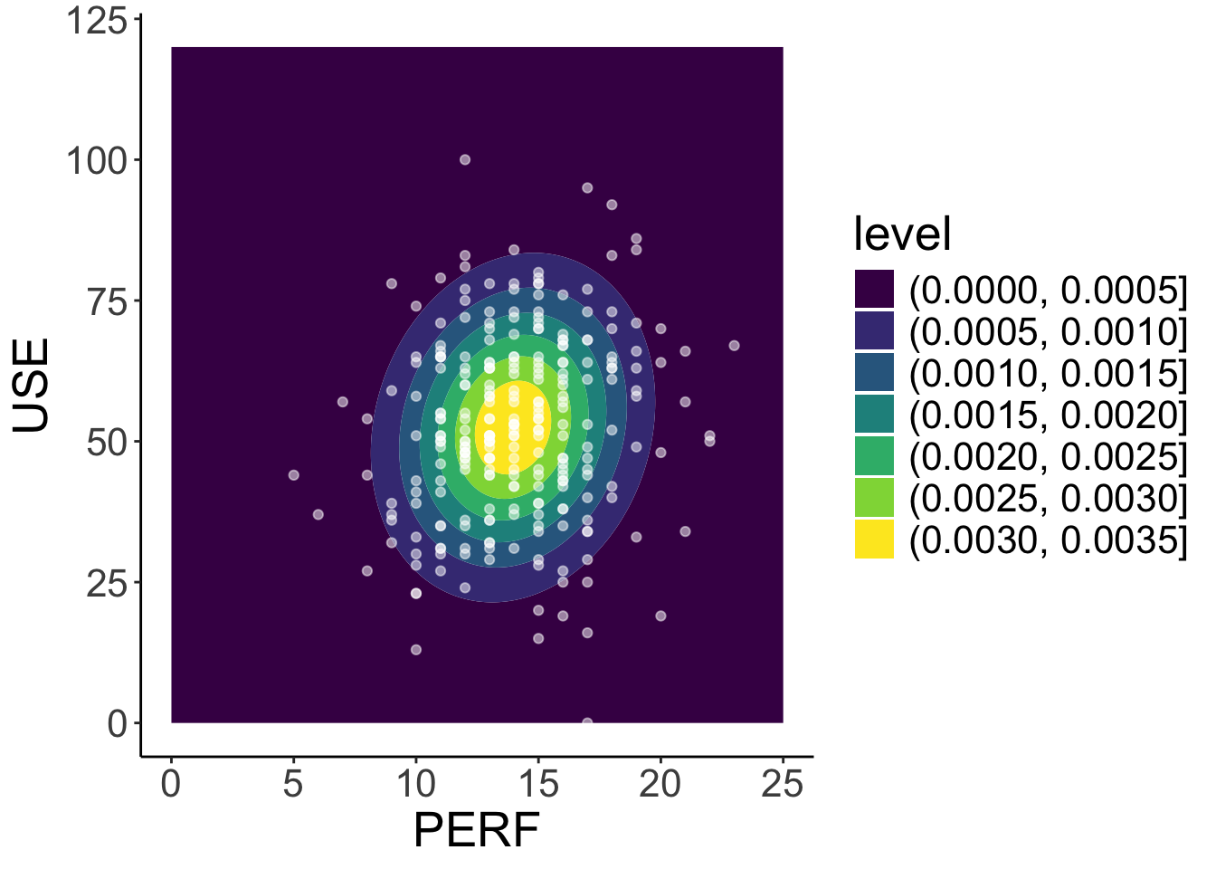
- We can use our estimated parameters to simulate the model-implied density plot for
perfanduse, which can be compared to the observed data forperfanduse.
Mutivariate normal density function
\begin{bmatrix}\text{PERF}_i\\\text{USE}_i\end{bmatrix} \sim \mathbf{N}_2 (\boldsymbol{\mu}_i=\begin{bmatrix}13.959\\52.440\end{bmatrix}, \mathbf{V}_i =\mathbf{R}=\begin{bmatrix}8.742 & 6.847\\ 6.847 & 249.245 \end{bmatrix})
⌘+C
library(plotly)
density_surface <- sim_dat |>
pivot_wider(names_from = use, values_from = density) |>
select(-perf) |>
as.matrix()
plot_ly(z = density_surface, x = seq(0, 120, .1), y = seq(0, 25, .1), colors = "PuRd", color = "green",
width = 1600, height = 800) |> add_surface()