?mean浪漫主义者的学R之旅-2
教程
0. 查阅文档
可以使用?fun()或者help(fun)的方式来查阅帮助文档。如果使用Rstudio的话,帮助文档会以html的格式出现在Viewer里。
1. 描述性统计
首先,安装以下R包。dplyr是一个优秀的数据分析处理的包,它的作者是Hadley Wickham。你可以浏览这个网页来了解更多dplyr的使用方法。本文之所以使用这个包而非R basic functions是因为我认为越早接触杰出的高级包可以减少以后重新学习的时间成本。毕竟R基础的方法(functions)实在是限制太多,需要很长时间的积累才能够进行数据处理。而dplyr只要掌握了基础的操作就发现数据处理很简单。而且,你可以通过点击RStudio上方菜单上的 Help > Cheatsheats > Data Transformation with dplyr 就可以查看它的使用方法,十分方便。
usefulR是我制作的,方便初学者使用的R包。里面储存了一些示例数据。
## check if install packages
is_inst <- function(pkg) {
    nzchar(system.file(package = pkg))
}
if (!is_inst("usefulR")) { devtools::install_github("jihongz/usefulR")}
if (!is_inst("dplyr")) { install.packages("dplyr") }

## load packages
library(usefulR)
library(dplyr)
1.1 本文数据
我制作了一个伪教育数据SimpleEduData。共有100行,3列。教育数据常见的格式为一列数据代表一道题的所有答案(item),一行数据代表一个学生在这三道题上的得分。得分的分值最小为1,最大为6。
1.2 检查数据
1.2.1 行数据:部分查看
首先,由于通常你收到的数据的数据量都会很大,没有必要打开Excel一一查看所有数据。在R中,你可以使用head(data)或tail(data)快速查看数据的头六行和最后六行。dplyr提供了一个更方便的函数sample_n来随机查看几行数据。举例来看,第一个学生(row1)分别第一、二、三题答了3、1、4分;最后一个学生分别答了6、1、1分。
head(SimpleEduData) item1 item2 item3
1 3 1 4
2 5 4 1
3 2 5 1
4 3 3 2
5 1 1 3
6 2 4 1tail(SimpleEduData) item1 item2 item3
95 3 1 2
96 3 1 2
97 5 2 1
98 2 1 3
99 3 6 1
100 6 1 1sample_n(SimpleEduData, 6) item1 item2 item3
1 3 3 2
2 3 1 4
3 6 1 1
4 4 5 1
5 3 3 1
6 1 5 21.2.2 列数据:图表查看
如果你想要查看一列数据(column)的话,我推荐使用箱形图(boxplot)或者直方图(histogram)的方式来给自己初步的分析。
par(mfrow=c(2,2))

plot_histgram <- function(onecolumn) {
  hist(onecolumn, breaks = (c(1:7)-0.5), col = 'lightblue', border = "darkblue")
}
plot_histgram(SimpleEduData$item1)
hist(SimpleEduData$item2, breaks = (c(1:7)-0.5))
hist(SimpleEduData$item3, breaks = (c(1:7)-0.5))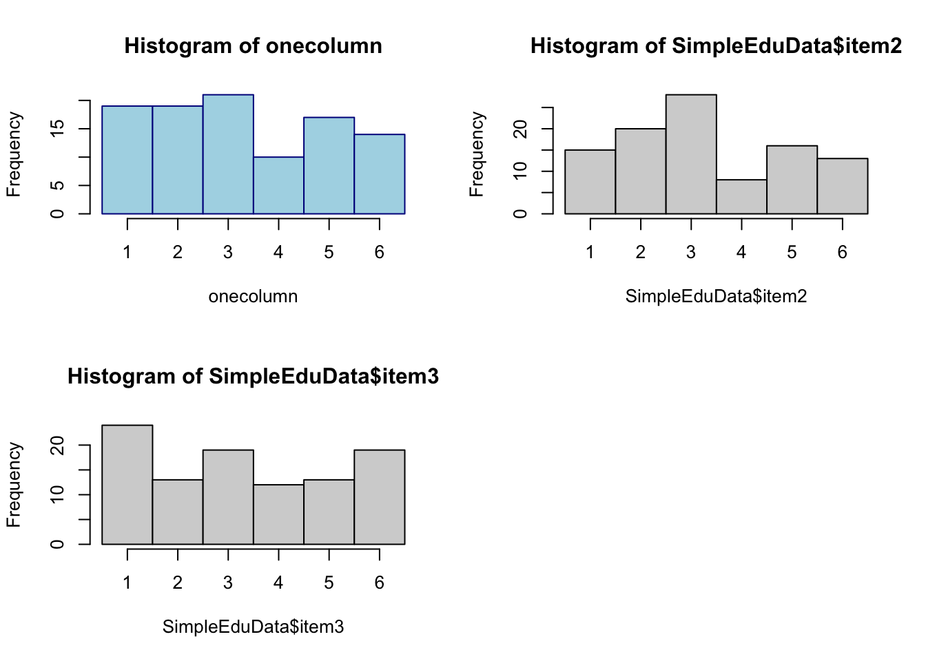
或者你也可以用ggplot2包来创造更复杂的直方图。
## 增加density plot
library(ggplot2)
ggplot(data = SimpleEduData) +
  geom_histogram(aes(item2, y = ..density..), breaks = (c(1:7)-0.5),col = "skyblue", fill = "red3") +
  geom_density(aes(item2), position = "stack")
Warning: The dot-dot notation (`..density..`) was deprecated in ggplot2 3.4.0.
ℹ Please use `after_stat(density)` instead.
plotdata <- SimpleEduData %>%
  gather(item, value)

## Prepare for Normal Distribution Density
grid <- with(plotdata, seq(min(value), max(value), length = 100))
normaldens <- ddply(plotdata, "item", function(df) {
  data.frame(
    predicted = grid,
    density = dnorm(grid, mean(df$value), sd(df$value))
  )
})

plotdata %>%
  ggplot(aes(x = value)) +
  geom_histogram(aes(y = ..density.., fill = item),
                 col = "white", binwidth = 1) +
  ## Add some lables for each bin
  stat_bin(binwidth=1, geom="text", colour="white", size=3,
           aes(label = ..count.., y = ..density..),
           position = position_stack(vjust=0.5)) +
  ## Add density line
  stat_density(geom = 'line', position = "stack",
               alpha = 0.5, adjust = 1, linetype = 3) +
  scale_x_continuous("Responses", limits = c(0,7),
                     labels = 1:6, breaks = 1:6) +
  scale_y_continuous("Frequency", limits = c(0,0.3),
                     labels = 0:6/20, breaks = 0:6/20) +
  ## Add normal density line
  geom_line(aes(y = density, x = predicted), data = normaldens, colour = c("#082F45")) +
  facet_wrap(~item, nrow = 2) +
  scale_fill_brewer(palette = "Set2") +
  theme_light()
Warning: Removed 6 rows containing missing values or values outside the scale range
(`geom_bar()`).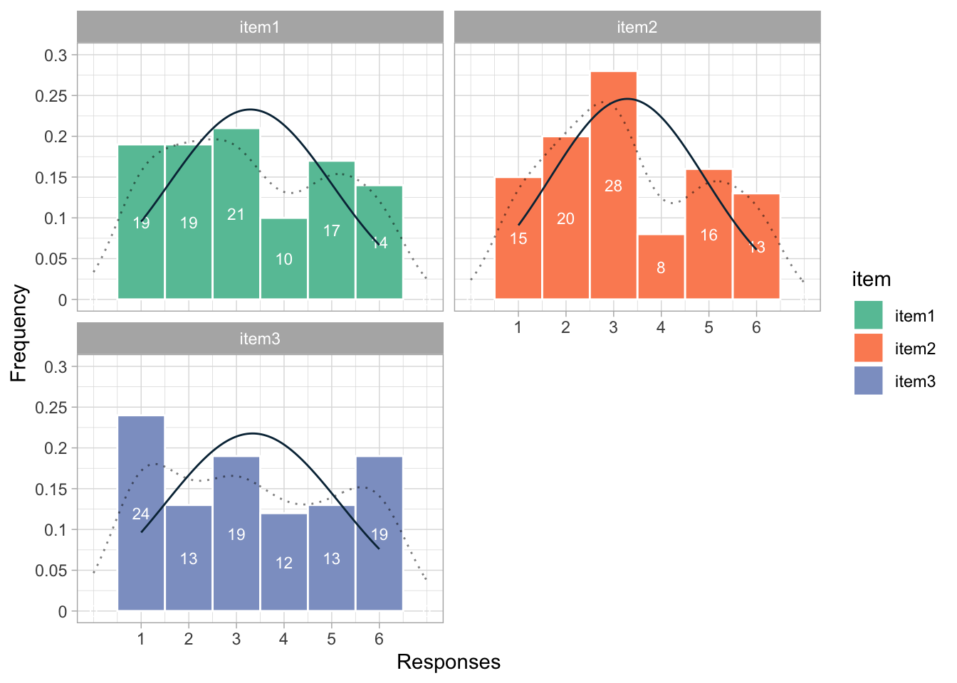
par(mfrow=c(2,2))
boxplot(SimpleEduData$item1)
title("Item1")
boxplot(SimpleEduData$item2)
title("Item2")
boxplot(SimpleEduData$item3)
title("Item3")
1.2.3 检查缺失值
summary(SimpleEduData) item1 item2 item3
Min. :1.00 Min. :1.00 Min. :1.00
1st Qu.:2.00 1st Qu.:2.00 1st Qu.:2.00
Median :3.00 Median :3.00 Median :3.00
Mean :3.29 Mean :3.29 Mean :3.34
3rd Qu.:5.00 3rd Qu.:5.00 3rd Qu.:5.00
Max. :6.00 Max. :6.00 Max. :6.00# Add some missing values
SimpleEduData_missing <- data.frame(rbind(SimpleEduData, c(NA,NA,NA)))
tail(SimpleEduData_missing) item1 item2 item3
96 3 1 2
97 5 2 1
98 2 1 3
99 3 6 1
100 6 1 1
101 NA NA NAsummary(SimpleEduData_missing) item1 item2 item3
Min. :1.00 Min. :1.00 Min. :1.00
1st Qu.:2.00 1st Qu.:2.00 1st Qu.:2.00
Median :3.00 Median :3.00 Median :3.00
Mean :3.29 Mean :3.29 Mean :3.34
3rd Qu.:5.00 3rd Qu.:5.00 3rd Qu.:5.00
Max. :6.00 Max. :6.00 Max. :6.00
NA's :1 NA's :1 NA's :11.3 数据运算
1.3.1 求和
每一行的和可以用rowSums()函数来求和,有时候如果有missing values则要加上na.rm = TRUE的argument。
rowSums(SimpleEduData)
rowSums(SimpleEduData, na.rm = TRUE)另外,一个常见的做法是新建一个变量来储存总和。具体来说,total是每一个学生三道题的总分。
SimpleEduData %>%
  mutate(total = rowSums(.)) %>%
  head(10)
item1 item2 item3 total
1 3 1 4 8
2 5 4 1 10
3 2 5 1 8
4 3 3 2 8
5 1 1 3 5
6 2 4 1 7
7 3 3 1 7
8 6 5 5 16
9 5 2 3 10
10 5 5 3 13SimpleEduData %>%
.[1:8, ] item1 item2 item3
1 3 1 4
2 5 4 1
3 2 5 1
4 3 3 2
5 1 1 3
6 2 4 1
7 3 3 1
8 6 5 5SimpleEduData %>%
mutate(id = rownames(.)) %>%
filter(item1 == 6, item2 ==1, item3 ==1) item1 item2 item3 id
1 6 1 1 85
2 6 1 1 100SimpleEduData %>%
mutate(sex = c(rep(0, 50), rep(1, 50))) %>%
mutate(total = rowSums(.)) %>%
group_by(sex) %>%
summarise(Meantotalscore = mean(total), meanitem1 = mean(item1), meanitem2 = mean(item2)) Meantotalscore meanitem1 meanitem2
1 10.42 3.29 3.29library(dplyr)
library(usefulR)
system.time(usefulR::frequency_table(SimpleEduData)) user system elapsed
0.003 0.000 0.004system.time(summary(SimpleEduData)) user system elapsed
0.000 0.000 0.001