[1] 0.6Bayes’ Theorem
Likelihood function, Posterior distribution
How to report posterior distribution of parameters
Bayesian update
but, before we begin…
Bayesian methods rely on Bayes’ Theorem
P(\theta | Data) = \frac{P(Data|\theta)P(\theta)}{P(Data)} \propto P(Data|\theta) P(\theta)
Where:
Suppose we want to assess the probability of rolling a “1” on a six-sided die:
\theta \equiv p_{1} = P(D = 1)
Suppose we collect a sample of data (N = 5):
Data \equiv X = \{0, 1, 0, 1, 1\}
The prior distribution of parameters is denoted as P(p_1) ;
The likelihood functionis denoted as P(X | p_1);
The posterior distribution is denoted as P(p_1|X)
Then we have:
P(p_1|X) = \frac{P(X|p_1)P(p_1)}{P(X)} \propto P(X|p_1) P(p_1)

The Likelihood function P(X|p_1) follows Binomial distribution of 3 succuess out of 5 samples:
P(X|p_1) = \prod_{i =1}^{N=5} p_1^{X_i}(1-p_1)^{X_i}
\\= (1-p_i) \cdot p_i \cdot (1-p_i) \cdot p_i \cdot p_i
Question here: WHY use Bernoulli (Binomial) Distribution (feat. Jacob Bernoulli, 1654-1705)?
My answer: Bernoulli dist. has nice statistical probability. “Nice” means making totally sense in normal life– a common belief. For example, the p_1 value that maximizes the Bernoulli-based likelihood function is Mean(X), and the p_1 values that minimizes the Bernoulli-based likelihood function is 0 or 1
Assume each event is independent, the multiplication of the probabilities of each event is the “Likelihood”. Log transform of Likelihood is easier for further analysis.
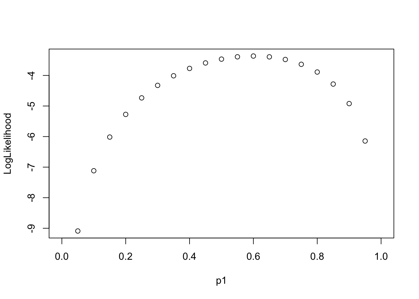
LL(p_1|\{0, 1, 0, 1, 1\})
Goal: find the most possible p1 value (the probability of the event) so that the data {0, 1, 0, 1, 1} has the highest likelihood
[1] 0.6LL(Data|p_1 \in \{0, 0.2,0.4, 0.6, 0.8,1\})
library(tidyverse)
p1 = c(0, 2, 4, 6, 8, 10) / 10
nTrails = 5
nSuccess = 0:nTrails
Likelihood = sapply(p1, \(x) choose(nTrails,nSuccess)*(x)^nSuccess*(1-x)^(nTrails - nSuccess))
Likelihood_forPlot <- as.data.frame(Likelihood)
colnames(Likelihood_forPlot) <- p1
Likelihood_forPlot$Sample = factor(paste0(nSuccess, " out of ", nTrails), levels = paste0(nSuccess, " out of ", nTrails))
# plot
Likelihood_forPlot %>%
  pivot_longer(-Sample, names_to = "p1") %>%
  mutate(`log(Likelihood)` = log(value)) %>%
  ggplot(aes(x = Sample, y = `log(Likelihood)`, color = p1)) +
  geom_point(size = 2) +
  geom_path(aes(group=p1), size = 1.3)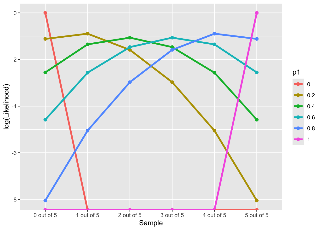
We must now pick the prior distribution of p_1:
P(p_1)
Compared to likelihood function, we have much more choices. Many distributions to choose from
To choose prior distribution, think about what we know about a “fair” die.
the probability of rolling a “1” is about \frac{1}{6}
the probabilities much higher/lower than \frac{1}{6} are very unlikely
Let’s consider a Beta distribution as the prior distribution of p_1:
p_1 \sim Beta(\alpha, \beta)
or
P(p_1) \equiv Beta(\alpha, \beta)
For parameters that range between 0 and 1, the beta distribution makes a good choice for prior distribution:
P(p_1) = \frac{(p_1)^{a-1} (1-p_1)^{\beta-1}}{B(\alpha,\beta)}
Where denominator, B, is a normalization constant to ensure that the total probability is 1:
B(\alpha,\beta) = \frac{\Gamma(\alpha)\Gamma(\beta)}{\Gamma(\alpha+\beta)}
and (fun fact: derived by Daniel Bernoulli (1700-1782)),
\Gamma(\alpha) = \int_0^{\infty}t^{\alpha-1}e^{-t}dt
Think about 3 sets of 10 dices. They have varied probability of “1”.
Question1: any fair dice among 30 dices?
Question2: which set have relatively fair dices.
Hint: 1 / 6 = 0.16666...
set.seed(4)
alpha = 2
beta = 2
rbeta(n = 10, shape1 = alpha, shape2 = beta) # randomly generate p1 given beta(2, 2)
[1] 0.5609713 0.3497046 0.7392076 0.6644891 0.8877412 0.6888135 0.4400386
[8] 0.9230177 0.9079563 0.5044343alpha = 1
beta = 1
rbeta(n = 10, shape1 = alpha, shape2 = beta) # randomly generate p1 given beta(1, 1) [1] 0.35083863 0.51800100 0.48629826 0.43288779 0.12200407 0.51762911
[7] 0.53997409 0.61158197 0.06168091 0.43440547alpha = 200
beta = 996
rbeta(n = 10, shape1 = alpha, shape2 = beta) # randomly generate p1 given beta(200, 996) [1] 0.1851006 0.1746928 0.1637927 0.1842677 0.1790450 0.1558018 0.1840178
[8] 0.1691043 0.1580080 0.1483028The Beta distribution has a mean of \frac{\alpha}{\alpha+\beta} and a mode of \frac{\alpha -1}{\alpha + \beta -2} for \alpha > 1 & \beta > 1; (fun fact: when \alpha\ \&\ \beta< 1, pdf is U-shape, what that mean?)
\alpha and \beta are called hyperparameters of the parameter p_1;
Hyperparameters are parameters of prior parameters ;
When \alpha = \beta = 1, the distribution is uniform distribution;
To make sure P(p_1 = \frac{1}{6}) is the largest, we can:
Many choices of prior distribution:
\alpha =2 and \beta = 6 has the same mode as \alpha = 100 and \beta = 496;
hint: when the relationship between \alpha and \eta follows \beta = 5\alpha - 4
The differences between choices is how strongly we feel in our beliefs
dbeta <- function(p1, alpha, beta) {
  # probability density function
  PDF = ((p1)^(alpha-1)*(1-p1)^(beta-1)) / beta(alpha, beta)
  return(PDF)
}

condition <- data.frame(
  alpha = c(2, 20, 100, 200),
  beta = c(6, 96, 496, 996)
)
pdf_bycond <- condition %>%
  nest_by(alpha, beta) %>%
  mutate(data = list(
    dbeta(p1 = (1:99)/100, alpha = alpha, beta = beta)
  ))

## prepare data for plotting pdf by conditions
pdf_forplot <- Reduce(cbind, pdf_bycond$data) %>%
  t() %>%
  as.data.frame() ## merge conditions together
colnames(pdf_forplot) <- (1:99)/100 # add p1 values as x-axis
pdf_forplot <- pdf_forplot %>%
  mutate(Alpha_Beta = c( # add alpha_beta conditions as colors
    "(2, 6)",
    "(20, 96)",
    "(100, 496)",
    "(200, 996)"
  )) %>%
  pivot_longer(-Alpha_Beta, names_to = 'p1', values_to = 'pdf') %>%
  mutate(p1 = as.numeric(p1),
         Alpha_Beta = factor(Alpha_Beta,levels = unique(Alpha_Beta)))

pdf_forplot %>%
  ggplot() +
  geom_vline(xintercept = 0.17, col = "black") +
  geom_point(aes(x = p1, y = pdf, col = Alpha_Beta)) +
  geom_path(aes(x = p1, y = pdf, col = Alpha_Beta, group = Alpha_Beta)) +
  scale_color_discrete(name = "Prior choices")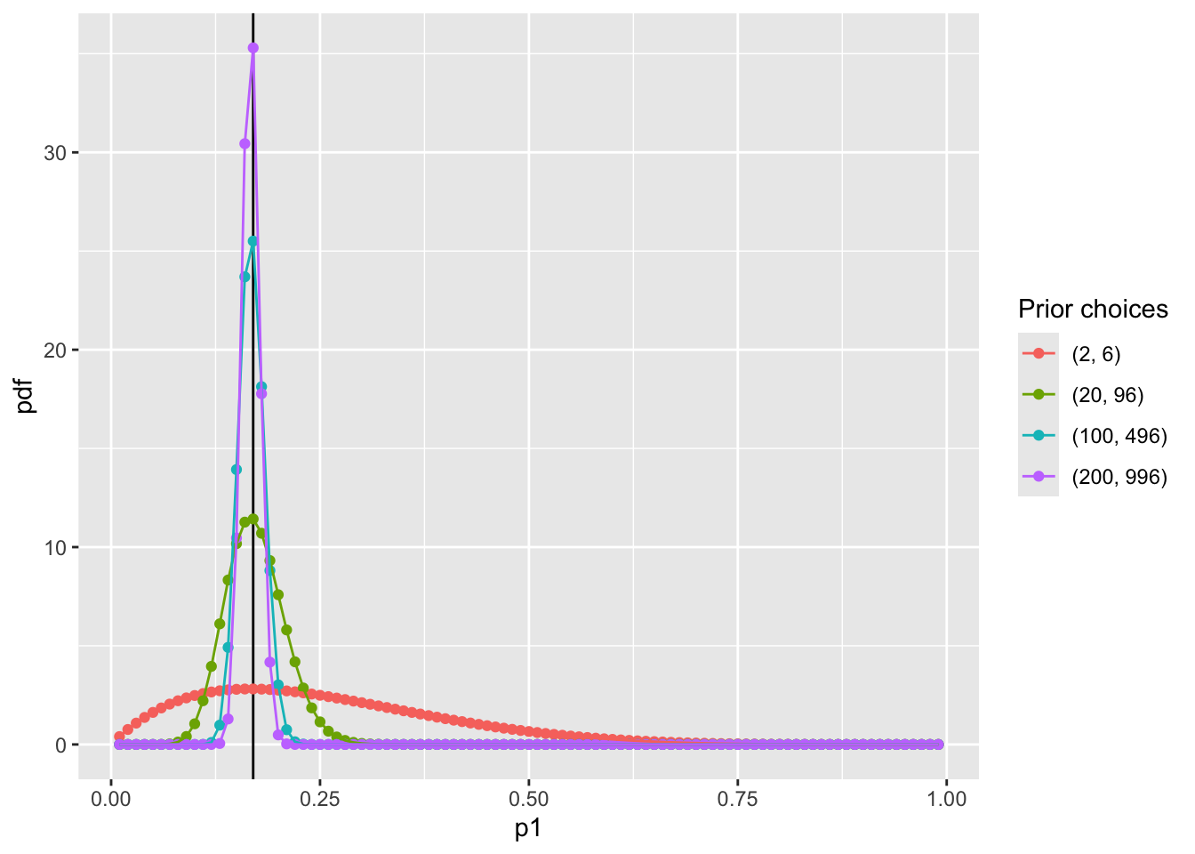
Question: WHY NOT USE NORMAL DISTRIBUTION?
# Function for variance of Beta distribution
varianceFun = function(alpha_beta){
  alpha = alpha_beta[1]
  beta = alpha_beta[2]
  return((alpha * beta)/((alpha + beta)^2*(alpha + beta + 1)))
}

# Multiple prior choices from uninformative to informative
alpha_beta_choices = list(
  I_dont_trust = c(2, 6),
  not_strong =   c(20, 96),
  litte_strong = c(100, 496),
  very_strong =  c(200, 996))

## Transform to data.frame for plot
alpha_beta_variance_plot <- t(sapply(alpha_beta_choices, varianceFun)) %>%
  as.data.frame() %>%
  pivot_longer(everything(), names_to = "Degree", values_to = "Variance") %>%
  mutate(Degree = factor(Degree, levels = unique(Degree))) %>%
  mutate(Alpha_Beta = c(
    "(2, 6)",
    "(20, 96)",
    "(100, 496)",
    "(200, 996)"
  ))

alpha_beta_variance_plot %>%
  ggplot(aes(x = Degree, y = Variance)) +
  geom_col(aes(fill = Degree)) +
  geom_text(aes(label = Alpha_Beta), size = 6) +
  labs(title = "Variances along difference choices of alpha and beta") +
theme(text = element_text(size = 21)) 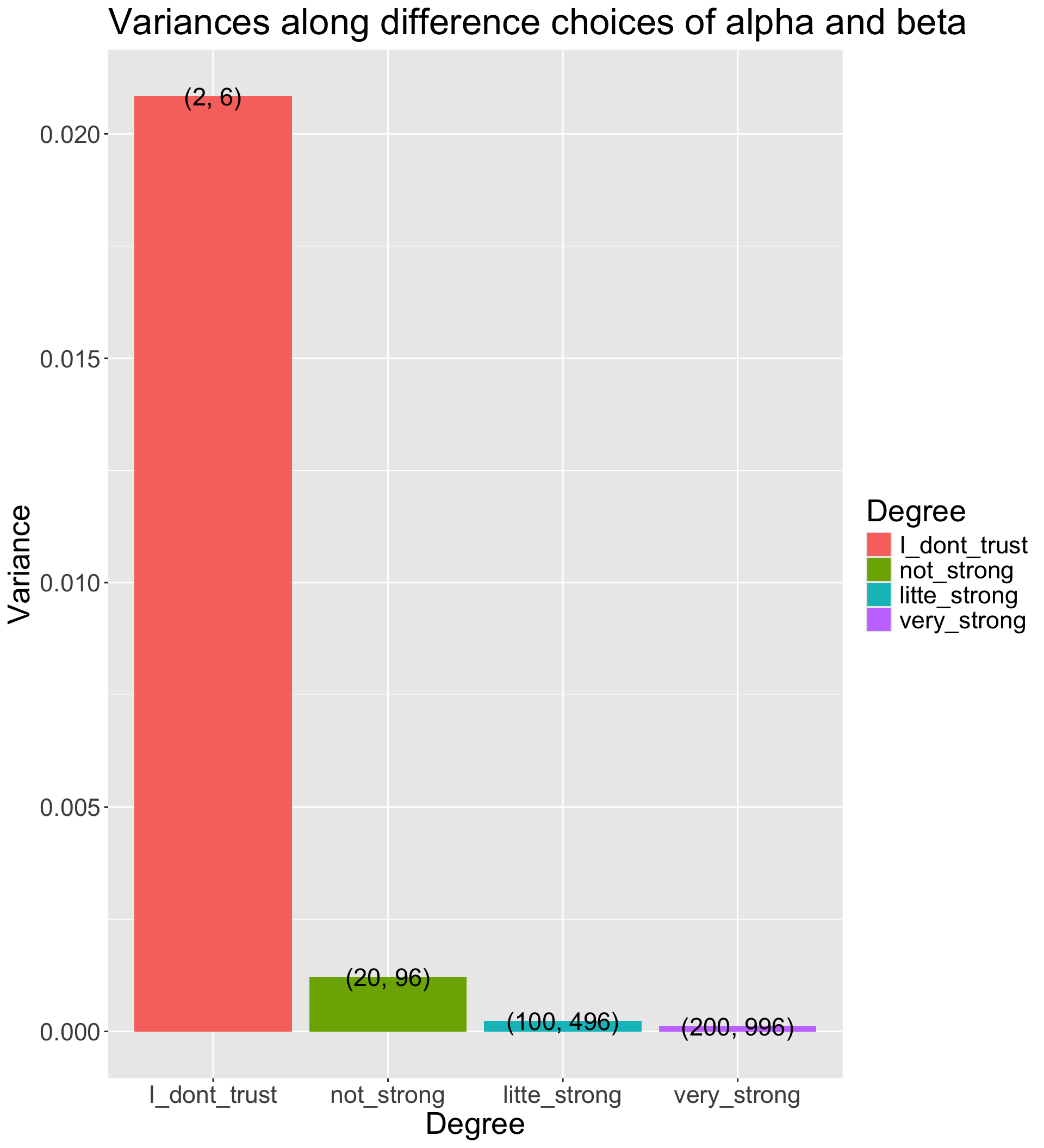
Choose a Beta distribution as the prior distribution of p_1 is very convenient:
When combined with Bernoulli (Binomial) data likelihood, the posterior distribution (P(p_1|Data)) can be derived analytically
The posterior distribution is also a Beta distribution
\alpha' = \alpha + \sum_{i=1}^{N}X_i (\alpha' is parameter of the posterior distribution)
\beta' = \beta + (N - \sum_{i=1}^{N}X_i) (\beta' is parameter of the posterior distribution)
The Beta distribution is said to be a conjugate prior in Bayesian analysis: A prior distribution that leads to posterior distribution of the same family
dbeta_posterior <- function(p1, alpha, beta, data) {
  alpha_new = alpha + sum(data)
  beta_new = beta + (length(data) - sum(data) )
  # probability density function
  PDF = ((p1)^(alpha_new-1)*(1-p1)^(beta_new-1)) / beta(alpha_new, beta_new)
  return(PDF)
}
# Observed data
dat = c(0, 1, 0, 1, 1)

condition <- data.frame(
  alpha = c(2, 20, 100, 200),
  beta = c(6, 96, 496, 996)
)

pdf_posterior_bycond <- condition %>%
  nest_by(alpha, beta) %>%
  mutate(data = list(
    dbeta_posterior(p1 = (1:99)/100, alpha = alpha, beta = beta,
                    data = dat)
  ))

## prepare data for plotting pdf by conditions
pdf_posterior_forplot <- Reduce(cbind, pdf_posterior_bycond$data) %>%
  t() %>%
  as.data.frame() ## merge conditions together
colnames(pdf_posterior_forplot) <- (1:99)/100 # add p1 values as x-axis
pdf_posterior_forplot <- pdf_posterior_forplot %>%
  mutate(Alpha_Beta = c( # add alpha_beta conditions as colors
    "(2, 6)",
    "(20, 96)",
    "(100, 496)",
    "(200, 996)"
  )) %>%
  pivot_longer(-Alpha_Beta, names_to = 'p1', values_to = 'pdf') %>%
  mutate(p1 = as.numeric(p1),
         Alpha_Beta = factor(Alpha_Beta,levels = unique(Alpha_Beta)))

pdf_posterior_forplot %>%
  ggplot() +
  geom_vline(xintercept = 0.17, col = "black") +
  geom_point(aes(x = p1, y = pdf, col = Alpha_Beta)) +
  geom_path(aes(x = p1, y = pdf, col = Alpha_Beta, group = Alpha_Beta)) +
  scale_color_discrete(name = "Prior choices") +
  labs( y = '')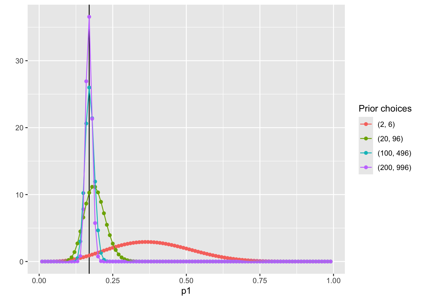
To determine the estimate of p_1, we need to summarize the posterior distribution:
With prior hyperparameters \alpha = 2 and \beta = 6:
\hat p_1 = \frac{2+3}{2+3+6+2}=\frac{5}{13} = .3846
SD = 0.1300237
With prior hyperparameters \alpha = 100 and \beta = 496:
\hat p_1 = \frac{100+3}{100+3+496+2}=\frac{103}{601} = .1714
SD = 0.0153589
uninfo <- pdf_posterior_forplot %>% filter(Alpha_Beta == "(2, 6)")
paste0("Sample Posterior Mean: ", mean(uninfo$p1 * uninfo$pdf)) # .3885
[1] "Sample Posterior Mean: 0.388500388484552"uninfo2 <- pdf_posterior_forplot %>% filter(Alpha_Beta == "(100, 496)")
paste0("Sample Posterior Mean: ", mean(uninfo2$p1 * uninfo2$pdf)) # 0.1731[1] "Sample Posterior Mean: 0.173112153145432"library(cmdstanr)
set_cmdstan_path("~/cmdstan/")
register_knitr_engine(override = FALSE)data {
int<lower=0> N; // sample size
array[N] int<lower=0, upper=1> y; // observed data
real<lower=1> alpha; // hyperparameter alpha
real<lower=1> beta; // hyperparameter beta
}
parameters {
real<lower=0,upper=1> p1; // parameters
}
model {
p1 ~ beta(alpha, beta); // prior distribution
for(n in 1:N){
y[n] ~ bernoulli(p1); // model
}
}# mod <- cmdstan_model('dice_model.stan')
data_list1 <- list(
y = c(0, 1, 0, 1, 1),
N = 5,
alpha = 2,
beta = 6
)
data_list2 <- list(
y = c(0, 1, 0, 1, 1),
N = 5,
alpha = 100,
beta = 496
)
fit1 <- dice_model$sample(
data = data_list1,
seed = 123,
chains = 4,
parallel_chains = 4,
refresh = 1000
)Running MCMC with 4 parallel chains...
Chain 1 Iteration: 1 / 2000 [ 0%] (Warmup)
Chain 1 Iteration: 1000 / 2000 [ 50%] (Warmup)
Chain 1 Iteration: 1001 / 2000 [ 50%] (Sampling)
Chain 1 Iteration: 2000 / 2000 [100%] (Sampling)
Chain 2 Iteration: 1 / 2000 [ 0%] (Warmup)
Chain 2 Iteration: 1000 / 2000 [ 50%] (Warmup)
Chain 2 Iteration: 1001 / 2000 [ 50%] (Sampling)
Chain 2 Iteration: 2000 / 2000 [100%] (Sampling)
Chain 3 Iteration: 1 / 2000 [ 0%] (Warmup)
Chain 3 Iteration: 1000 / 2000 [ 50%] (Warmup)
Chain 3 Iteration: 1001 / 2000 [ 50%] (Sampling)
Chain 3 Iteration: 2000 / 2000 [100%] (Sampling)
Chain 4 Iteration: 1 / 2000 [ 0%] (Warmup)
Chain 4 Iteration: 1000 / 2000 [ 50%] (Warmup)
Chain 4 Iteration: 1001 / 2000 [ 50%] (Sampling)
Chain 4 Iteration: 2000 / 2000 [100%] (Sampling)
Chain 1 finished in 0.0 seconds.
Chain 2 finished in 0.0 seconds.
Chain 3 finished in 0.0 seconds.
Chain 4 finished in 0.0 seconds.
All 4 chains finished successfully.
Mean chain execution time: 0.0 seconds.
Total execution time: 0.2 seconds.fit2 <- dice_model$sample(
data = data_list2,
seed = 123,
chains = 4,
parallel_chains = 4,
refresh = 1000
)Running MCMC with 4 parallel chains...
Chain 1 Iteration: 1 / 2000 [ 0%] (Warmup)
Chain 1 Iteration: 1000 / 2000 [ 50%] (Warmup)
Chain 1 Iteration: 1001 / 2000 [ 50%] (Sampling)
Chain 1 Iteration: 2000 / 2000 [100%] (Sampling)
Chain 2 Iteration: 1 / 2000 [ 0%] (Warmup)
Chain 2 Iteration: 1000 / 2000 [ 50%] (Warmup)
Chain 2 Iteration: 1001 / 2000 [ 50%] (Sampling)
Chain 2 Iteration: 2000 / 2000 [100%] (Sampling)
Chain 3 Iteration: 1 / 2000 [ 0%] (Warmup)
Chain 3 Iteration: 1000 / 2000 [ 50%] (Warmup)
Chain 3 Iteration: 1001 / 2000 [ 50%] (Sampling)
Chain 3 Iteration: 2000 / 2000 [100%] (Sampling)
Chain 4 Iteration: 1 / 2000 [ 0%] (Warmup)
Chain 4 Iteration: 1000 / 2000 [ 50%] (Warmup)
Chain 4 Iteration: 1001 / 2000 [ 50%] (Sampling)
Chain 4 Iteration: 2000 / 2000 [100%] (Sampling)
Chain 1 finished in 0.0 seconds.
Chain 2 finished in 0.0 seconds.
Chain 3 finished in 0.0 seconds.
Chain 4 finished in 0.0 seconds.
All 4 chains finished successfully.
Mean chain execution time: 0.0 seconds.
Total execution time: 0.2 seconds.bayesplot::mcmc_dens(fit1$draws('p1')) +
geom_path(aes(x = p1, y = pdf), data = pdf_posterior_forplot %>% filter(Alpha_Beta == '(2, 6)'), col = "red") +
geom_vline(xintercept = 1/6, col = "green") +
geom_vline(xintercept = 3/5, col = "purple") +
labs(title = "Posterior distribution using uninformative prior vs. the conjugate prior (The Gibbs sampler) method", caption = 'Green: mode of prior distribution; Purple: expected value from observed data; Red: Gibbs sampling method')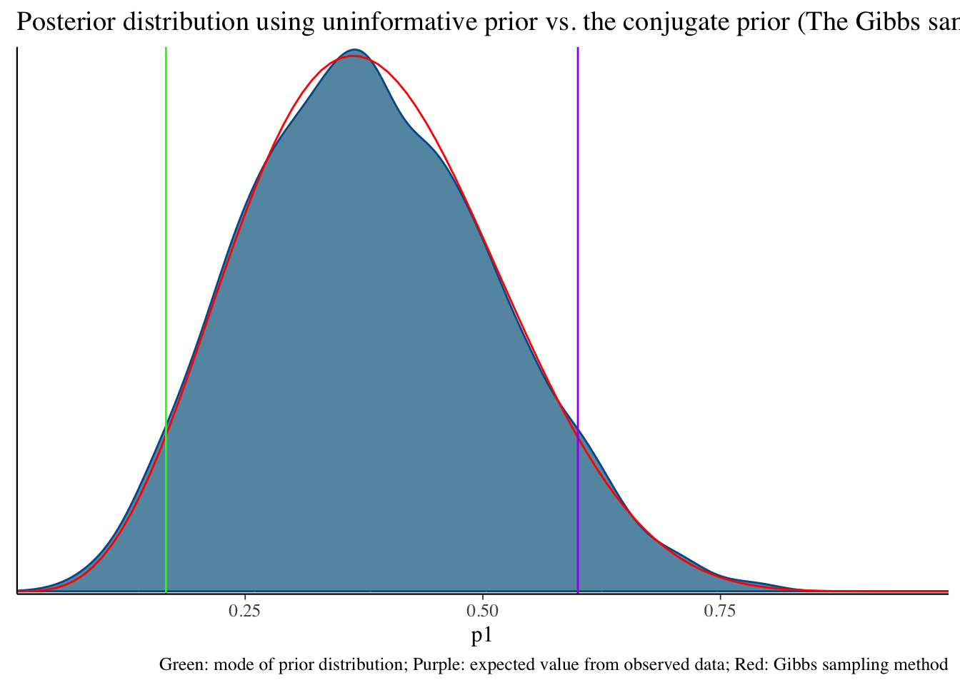
fit1$summary()# A tibble: 2 × 10
variable mean median sd mad q5 q95 rhat ess_bulk ess_tail
<chr> <dbl> <dbl> <dbl> <dbl> <dbl> <dbl> <dbl> <dbl> <dbl>
1 lp__ -9.19 -8.91 0.751 0.337 -10.7 -8.66 1.00 1812. 2400.
2 p1 0.383 0.377 0.131 0.137 0.180 0.609 1.00 1593. 1629.bayesplot::mcmc_dens(fit2$draws('p1')) +
geom_path(aes(x = p1, y = pdf), data = pdf_posterior_forplot %>% filter(Alpha_Beta == '(100, 496)'), col = "red") +
geom_vline(xintercept = 1/6, col = "green") +
geom_vline(xintercept = 3/5, col = "purple") +
labs(title = "Posterior distribution using informative prior vs. the conjugate prior (The Gibbs sampler) method", caption = 'Green: mode of prior distribution; Purple: expected value from observed data; Red: Gibbs sampling method')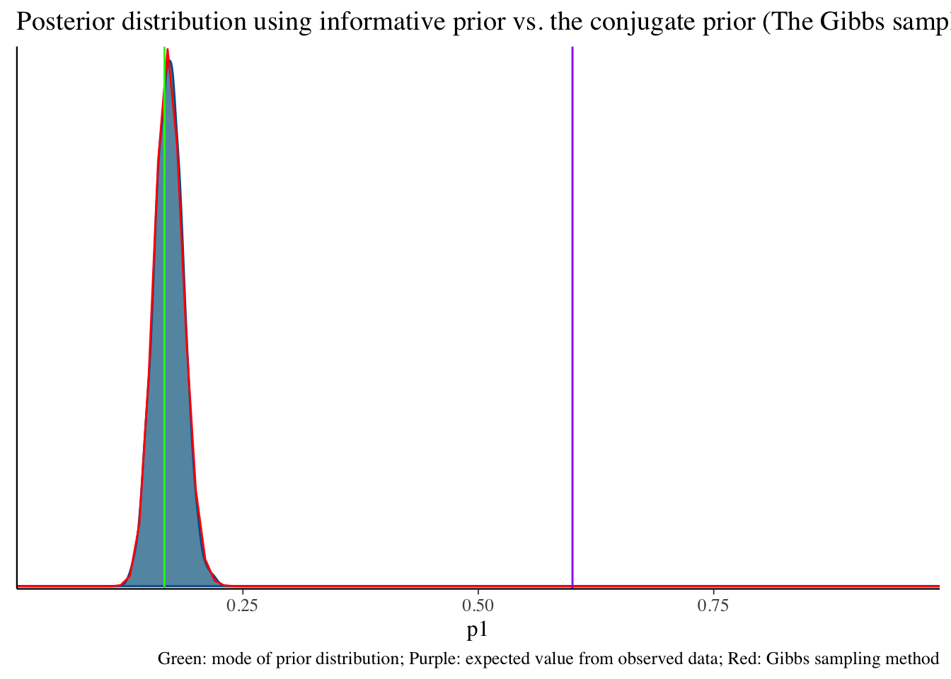
fit2$summary()# A tibble: 2 × 10
variable mean median sd mad q5 q95 rhat ess_bulk
<chr> <dbl> <dbl> <dbl> <dbl> <dbl> <dbl> <dbl> <dbl>
1 lp__ -276. -276. 0.716 0.317 -277. -275. 1.00 1816.
2 p1 0.171 0.171 0.0154 0.0155 0.146 0.197 1.00 1627.
# ℹ 1 more variable: ess_tail <dbl>Install cmdstan and cmdstanr
Practice beta prior distribution with hyperparameter {2, 3}, {10, 15}
Summarize the results
We will talk more about how Bayesian model works. Thank you.
When the binomial likelihood is multiplied by the beta prior, the result is proportional to another beta distribution:
This is the kernel of a beta distribution with updated parameters \alpha' = x + \alpha and \beta' = n - x + \beta. The fact that the posterior is still a beta distribution is what makes the beta distribution a conjugate prior for the binomial likelihood.
Human langauge: Both beta (prior) and binomial (likelihood) are so-called “exponetial family”. The muliplication of them is still a “exponential family” distribution.
We can use the posterior distribution as a prior!
1. data {0, 1, 0, 1, 1} with the prior hyperparameter {2, 6} -> posterior parameter {5, 9}
2. new data {1, 1, 1, 1, 1} with the prior hyperparameter {5, 9} -> posterior parameter {10, 9}
3. one more new data {0, 0, 0, 0, 0} with the prior hyperparameter {10, 9} -> posterior parameter {10, 14}
Today is a quick introduction to Bayesian Concept