x = 5
print_x <- function(x) {x = 3; return(x)}
x
[1] 5x = 5
print_x <- function(x) {x = 3; return(x)}
x[1] 5add <- function(x, y) {
result <- x + y
return(result)
}
add(2, 3) # Output: 5[1] 5result # Error: object 'result' not foundError: object 'result' not found<<- to copy the object result to the global enviroment.add <- function(x, y) {
result <<- x + y
return(result)
}
add(2, 3) # Output: 5[1] 5result [1] 5library(car)
m2 <- lm(prestige ~ education, data=carData::Prestige)
car::ncvTest(m2, ~ income)Non-constant Variance Score Test
Variance formula: ~ income
Chisquare = 1.520711, Df = 1, p = 0.21751This fits variable prestige as a linear function of predictor education, and tests for nonconstant variance as a function of income, another regressor in the data set Prestige.
lm when call it in the functionf3 <- function(meanmod, dta, varmod) {
m3 <- lm(meanmod, dta)
car::ncvTest(m3, varmod)
}
f3(meanmod=prestige ~ education, dta=carData::Prestige, varmod = ~ income)Error in eval(data, envir = environment(formula(model))): object 'dta' not foundlibrary(pryr) #install.packages("pryr")
f3_2 <- function(meanmod, dta, varmod) {
m3 <- lm(meanmod, dta)
print(environment(formula(m3))) # lm define formula in the global enviroment
where("dta")
}
f3_2(meanmod=prestige ~ education, dta=carData::Prestige, varmod = ~ income)<environment: R_GlobalEnv><environment: 0x10c449398>The arguments dta and meanmod are defined in the environment of the function, but the call to lm looks for them in the global environment, and they are therefore invisible when lm is called.
The assign function copies the dta and meanmod arguments to the global environment and rename them as .dta and .meanmod where ncvTest will be evaluated, and the remove function removes them before exiting the function.
f4 <- function(meanmod, dta, varmod) {
  assign(".dta", dta, envir=.GlobalEnv)
  m1 <- lm(meanmod, .dta)
  ans <- car::ncvTest(m1, varmod)
  remove(".dta", envir=.GlobalEnv)
  ans
}
f4(prestige ~ education, carData::Prestige, ~income)
Non-constant Variance Score Test
Variance formula: ~ income
Chisquare = 1.520711, Df = 1, p = 0.21751In this presentation, we will learn how to import data into R and tidy it for analysis.
Data is often messy, but understanding how to manipulate it is a critical skill for any data scientist.
While R packages provide a great way to work with sample data, at some point, you’ll need to apply what you’ve learned to your own data.
In today’s lecture, we’ll focus on importing rectangular data, especially CSV files.
A CSV (Comma Separated Values) file is a plain text file that contains tabular data, such as lists of information, in a format that can be easily read and written by humans and machines.
The values in each cell are separated by commas (hence the name), but other delimiters like semicolons, tabs, or pipes can also be used.
To read data in R, we’ll use the readr package, which is part of the tidyverse. Before you start, make sure to load the package.
library(tidyverse)
# or
library(readr)Let’s start with a common file format: CSV. Here’s a simple example:
Student ID,Full Name,favourite.food,mealPlan,AGE
1,Sunil Huffmann,Strawberry yoghurt,Lunch only,4
2,Barclay Lynn,French fries,Lunch only,5
3,Jayendra Lyne,N/A,Breakfast and lunch,7
4,Leon Rossini,Anchovies,Lunch only,
5,Chidiegwu Dunkel,Pizza,Breakfast and lunch,five
6,Güvenç Attila,Ice cream,Lunch only,6
You can read this CSV file into R using the read_csv() function.
students <- read_csv("data/students.csv")
students
# A tibble: 6 × 5
`Student ID` `Full Name` favourite.food mealPlan AGE
<dbl> <chr> <chr> <chr> <chr>
1 1 Sunil Huffmann Strawberry yoghurt Lunch only 4
2 2 Barclay Lynn French fries Lunch only 5
3 3 Jayendra Lyne N/A Breakfast and lunch 7
4 4 Leon Rossini Anchovies Lunch only <NA>
5 5 Chidiegwu Dunkel Pizza Breakfast and lunch five
6 6 Güvenç Attila Ice cream Lunch only 6 students$`Student ID`[1] 1 2 3 4 5 6"StudentID" # snake name[1] "StudentID"students_literal <- read_csv(I("
Student ID,Full Name,favourite.food,mealPlan,AGE
1,Sunil Huffmann,Strawberry yoghurt,Lunch only,4
2,Barclay Lynn,French fries,Lunch only,5
3,Jayendra Lyne,N/A,Breakfast and lunch,7
4,Leon Rossini,Anchovies,Lunch only,
5,Chidiegwu Dunkel,Pizza,Breakfast and lunch,five
6,Güvenç Attila,Ice cream,Lunch only,6"))
students_literal# A tibble: 6 × 5
`Student ID` `Full Name` favourite.food mealPlan AGE
<dbl> <chr> <chr> <chr> <chr>
1 1 Sunil Huffmann Strawberry yoghurt Lunch only 4
2 2 Barclay Lynn French fries Lunch only 5
3 3 Jayendra Lyne N/A Breakfast and lunch 7
4 4 Leon Rossini Anchovies Lunch only <NA>
5 5 Chidiegwu Dunkel Pizza Breakfast and lunch five
6 6 Güvenç Attila Ice cream Lunch only 6 read_delim as a more generic function to import data with customized deliminator.students_pipe <- read_delim(I("
Student ID|Full Name|favourite.food|mealPlan|AGE
1|Sunil Huffmann|Strawberry yoghurt|Lunch only|4
2|Barclay Lynn|French fries|Lunch only|5
3|Jayendra Lyne|N/A|Breakfast and lunch|7
4|Leon Rossini|Anchovies|Lunch only|
5|Chidiegwu Dunkel|Pizza|Breakfast and lunch|five
6|Güvenç Attila|Ice cream|Lunch only|6"), delim = "|")
students_pipe# A tibble: 6 × 5
`Student ID` `Full Name` favourite.food mealPlan AGE
<dbl> <chr> <chr> <chr> <chr>
1 1 Sunil Huffmann Strawberry yoghurt Lunch only 4
2 2 Barclay Lynn French fries Lunch only 5
3 3 Jayendra Lyne N/A Breakfast and lunch 7
4 4 Leon Rossini Anchovies Lunch only <NA>
5 5 Chidiegwu Dunkel Pizza Breakfast and lunch five
6 6 Güvenç Attila Ice cream Lunch only 6 If you want to copy this web Billboard Christian and Gospel table from Wikipedia, choose inspect from the right-clicked menu. Find the “<table>” html element, and copy outer HTML.
Install and Load rvest package
minimal_html: Convert the HTML text into html R object
html_element and html_table can convert the local html table into “tibble” format
library(rvest)
sample1 <- minimal_html('
<table class="wikitable sortable jquery-tablesorter">
<thead><tr>
<th width="200" class="headerSort" tabindex="0" role="columnheader button" title="Sort ascending">Chart title
</th>
<th width="120" class="headerSort" tabindex="0" role="columnheader button" title="Sort ascending">Chart type
</th>
<th class="headerSort" tabindex="0" role="columnheader button" title="Sort ascending"><small>Number of<br>positions</small>
</th>
<th class="unsortable">Description
</th></tr></thead><tbody>
<tr>
<td><a href="/wiki/Hot_Christian_Songs" title="Hot Christian Songs">Hot Christian Songs</a>
</td>
<td align="center">Sales, streaming, all format airplay
</td>
<td align="center">50
</td>
<td>Combines sales, airplay from all radio formats, and streaming data
</td></tr>
<tr>
<td>Christian Digital Song Sales
</td>
<td align="center">Digital downloads
</td>
<td align="center">50
</td>
<td>Top-downloaded <a href="/wiki/Christian_music" title="Christian music">Christian songs</a>, ranked by sales data as compiled by Luminate.
</td></tr>
<tr>
<td>Christian Streaming Songs
</td>
<td align="center">Streaming
</td>
<td align="center">50
</td>
<td>Most streamed Christian songs
</td></tr>
<tr>
<td><a href="/wiki/Christian_Airplay" title="Christian Airplay">Christian Airplay</a>
</td>
<td align="center">Airplay (audience)
</td>
<td align="center">50
</td>
<td>Audience impressions from Christian AC, Hot AC, CHR/Pop, Soft AC, and Christian Rock stations.
</td></tr>
<tr>
<td>Christian AC Airplay
</td>
<td align="center">Airplay (spins)
</td>
<td align="center">30
</td>
<td>Measures airplay spins on <a href="/wiki/Christian_adult_contemporary" title="Christian adult contemporary">Christian adult contemporary</a> stations
</td></tr>
<tr>
<td><a href="/wiki/Hot_Gospel_Songs" title="Hot Gospel Songs">Hot Gospel Songs</a>
</td>
<td align="center">Sales, streaming, allformat airplay
</td>
<td align="center">25
</td>
<td>Combines sales, airplay, and streaming data of Gospel songs
</td></tr>
<tr>
<td>Gospel Airplay
</td>
<td align="center">Radio (airplay)
</td>
<td align="center">30
</td>
<td>Measures airplay spins of Gospel stations
</td></tr>
<tr>
<td>Gospel Digital Song Sales
</td>
<td align="center">Digital sales
</td>
<td align="center">25
</td>
<td>Top-downloaded Gospel songs, ranked by sales data as compiled by Luminate.
</td></tr>
<tr>
<td>Gospel Streaming Songs
</td>
<td align="center">Streaming
</td>
<td align="center">15
</td>
<td>Top-streamed Gospel songs, ranked by sales data as compiled by Luminate.
</td></tr></tbody><tfoot></tfoot></table>  '
)
sample1 |>
  html_element("table") |>
  html_table()
# A tibble: 9 × 4
`Chart title` `Chart type` `Number ofpositions` Description
<chr> <chr> <int> <chr>
1 Hot Christian Songs Sales, streamin… 50 Combines s…
2 Christian Digital Song Sales Digital downloa… 50 Top-downlo…
3 Christian Streaming Songs Streaming 50 Most strea…
4 Christian Airplay Airplay (audien… 50 Audience i…
5 Christian AC Airplay Airplay (spins) 30 Measures a…
6 Hot Gospel Songs Sales, streamin… 25 Combines s…
7 Gospel Airplay Radio (airplay) 30 Measures a…
8 Gospel Digital Song Sales Digital sales 25 Top-downlo…
9 Gospel Streaming Songs Streaming 15 Top-stream…Try to import R&B and HipHop Table form Wikipedia to R.
# A tibble: 16 × 4
   `Chart title`                   `Chart type` `Number ofpositions` Description
   <chr>                           <chr>        <chr>                <chr>
 1 Hot R&B/Hip-Hop Songs           airplay + s… "50[A]"              Ranks the …
 2 R&B/Hip-Hop Airplay             airplay (au… "50"                 Measures a…
 3 R&B/Hip-Hop Digital Song Sales  digital sal… ""                   Top-downlo…
 4 R&B/Hip-Hop Streaming Songs     streaming    ""                   Top-stream…
 5 Mainstream R&B/Hip-Hop Airplay  airplay (sp… "40"                 Ranks song…
 6 Adult R&B Airplay               airplay (sp… "30"                 Measures a…
 7 Rhythmic Airplay                airplay (sp… "40"                 Measures a…
 8 Hot Rap Songs                   airplay + s… "25"                 Ranks the …
 9 Rap Airplay                     airplay (sp… "25"                 Ranks the …
10 Rap Digital Song Sales          digital sal… ""                   Top-downlo…
11 Rap Streaming Songs             streaming    ""                   Top-stream…
12 Hot R&B/Hip-Hop Recurrents      airplay (sp… "20"                 Ranks song…
13 Hot R&B/Hip-Hop Recurrent Airp… airplay (sp… "20"                 Ranks the …
14 Hot R&B Songs                   airplay + s… "25"                 Ranks the …
15 R&B Digital Song Sales          digital sal… ""                   Top-downlo…
16 R&B Streaming Songs streaming "" Top-stream…After loading your data, you’ll typically need to transform it for easier analysis. For instance, handling missing values is essential.
  students_fixedNA <- read_csv("data/students.csv", na = c("N/A", ""))
students_fixedNA
# A tibble: 6 × 5
`Student ID` `Full Name` favourite.food mealPlan AGE
<dbl> <chr> <chr> <chr> <chr>
1 1 Sunil Huffmann Strawberry yoghurt Lunch only 4
2 2 Barclay Lynn French fries Lunch only 5
3 3 Jayendra Lyne <NA> Breakfast and lunch 7
4 4 Leon Rossini Anchovies Lunch only <NA>
5 5 Chidiegwu Dunkel Pizza Breakfast and lunch five
6 6 Güvenç Attila Ice cream Lunch only 6 In some cases, column names may contain spaces, making them non-syntactic in R. You can handle this by renaming columns:
students_fixedColNames <- students |>
  rename(
    student_id = `Student ID`,
    full_name = `Full Name`,
    favourite_food = `favourite.food`,
    meal_plan = `mealPlan`
  )
students_fixedColNames
# A tibble: 6 × 5
student_id full_name favourite_food meal_plan AGE
<dbl> <chr> <chr> <chr> <chr>
1 1 Sunil Huffmann Strawberry yoghurt Lunch only 4
2 2 Barclay Lynn French fries Lunch only 5
3 3 Jayendra Lyne N/A Breakfast and lunch 7
4 4 Leon Rossini Anchovies Lunch only <NA>
5 5 Chidiegwu Dunkel Pizza Breakfast and lunch five
6 6 Güvenç Attila Ice cream Lunch only 6 janitor::clean_names() function for quick renaming. clean_names() use some heuristics to turn them all into snake case at once1.students |> janitor::clean_names()# A tibble: 6 × 5
student_id full_name favourite_food meal_plan age
<dbl> <chr> <chr> <chr> <chr>
1 1 Sunil Huffmann Strawberry yoghurt Lunch only 4
2 2 Barclay Lynn French fries Lunch only 5
3 3 Jayendra Lyne N/A Breakfast and lunch 7
4 4 Leon Rossini Anchovies Lunch only <NA>
5 5 Chidiegwu Dunkel Pizza Breakfast and lunch five
6 6 Güvenç Attila Ice cream Lunch only 6 Ensure that the variables are of the correct type. For example, the meal_plan column is categorical and should be a factor:
students_fixedDataType <- students_fixedColNames |>
  mutate(meal_plan = factor(meal_plan))
students_fixedDataType
# A tibble: 6 × 5
student_id full_name favourite_food meal_plan AGE
<dbl> <chr> <chr> <fct> <chr>
1 1 Sunil Huffmann Strawberry yoghurt Lunch only 4
2 2 Barclay Lynn French fries Lunch only 5
3 3 Jayendra Lyne N/A Breakfast and lunch 7
4 4 Leon Rossini Anchovies Lunch only <NA>
5 5 Chidiegwu Dunkel Pizza Breakfast and lunch five
6 6 Güvenç Attila Ice cream Lunch only 6 str(students_fixedDataType)tibble [6 × 5] (S3: tbl_df/tbl/data.frame)
$ student_id : num [1:6] 1 2 3 4 5 6
$ full_name : chr [1:6] "Sunil Huffmann" "Barclay Lynn" "Jayendra Lyne" "Leon Rossini" ...
$ favourite_food: chr [1:6] "Strawberry yoghurt" "French fries" "N/A" "Anchovies" ...
$ meal_plan : Factor w/ 2 levels "Breakfast and lunch",..: 2 2 1 2 1 2
$ AGE : chr [1:6] "4" "5" "7" NA ...table(students_fixedDataType$meal_plan)
Breakfast and lunch          Lunch only
2 4 Sometimes, your data is split across multiple files. You can read them all at once and combine them into a single data frame:
#| code-summary: "01-sales.csv"
#| code-fold: true
month,year,brand,item,n
January,2019,1,1234,3
January,2019,1,8721,9
January,2019,1,1822,2
January,2019,2,3333,1
January,2019,2,2156,9
January,2019,2,3987,6
January,2019,2,3827,6
#| code-summary: "02-sales.csv"
#| code-fold: true
month,year,brand,item,n
February,2019,1,1234,8
February,2019,1,8721,2
February,2019,1,1822,3
February,2019,2,3333,1
February,2019,2,2156,3
February,2019,2,3987,6#| code-summary: "03-sales.csv"
#| code-fold: true
month,year,brand,item,n
March,2019,1,1234,3
March,2019,1,3627,1
March,2019,1,8820,3
March,2019,2,7253,1
March,2019,2,8766,3
March,2019,2,8288,6sales_files <- c("data/01-sales.csv", "data/02-sales.csv", "data/03-sales.csv")
sales_data <- read_csv(sales_files, id = "file")
sales_data# A tibble: 19 × 6
file month year brand item n
<chr> <chr> <dbl> <dbl> <dbl> <dbl>
1 data/01-sales.csv January 2019 1 1234 3
2 data/01-sales.csv January 2019 1 8721 9
3 data/01-sales.csv January 2019 1 1822 2
4 data/01-sales.csv January 2019 2 3333 1
5 data/01-sales.csv January 2019 2 2156 9
6 data/01-sales.csv January 2019 2 3987 6
7 data/01-sales.csv January 2019 2 3827 6
8 data/02-sales.csv February 2019 1 1234 8
9 data/02-sales.csv February 2019 1 8721 2
10 data/02-sales.csv February 2019 1 1822 3
11 data/02-sales.csv February 2019 2 3333 1
12 data/02-sales.csv February 2019 2 2156 3
13 data/02-sales.csv February 2019 2 3987 6
14 data/03-sales.csv March 2019 1 1234 3
15 data/03-sales.csv March 2019 1 3627 1
16 data/03-sales.csv March 2019 1 8820 3
17 data/03-sales.csv March 2019 2 7253 1
18 data/03-sales.csv March 2019 2 8766 3
19 data/03-sales.csv March 2019 2 8288 6This will add a new column identifying which file the data came from.
You can also write data back to a file. For example, save the students data frame as a CSV:
write_csv(students_fixedDataType, "data/students_final.csv")For more complex objects, consider using write_rds() for saving R-specific objects.
Once you’ve mastered read_csv(), using readr’s other functions is straightforward; it’s just a matter of knowing which function to reach for:
read_csv2() reads semicolon-separated files. These use ; instead of , to separate fields and are common in countries that use , as the decimal marker.
read_tsv() reads tab-delimited files.
read_delim() reads in files with any delimiter, attempting to automatically guess the delimiter if you don’t specify it.
read_fwf() reads fixed-width files. You can specify fields by their widths with fwf_widths() or by their positions with fwf_positions().
read_table() reads a common variation of fixed-width files where columns are separated by white space.
read_log() reads Apache-style log files.
The readxl package provides functions to read-in Microsoft Excel formats.
The Microsoft Excel formats permit you to have more than one spreadsheet in one file.
These are referred to as sheets. The functions listed above read the first sheet by default, but we can also read the others by specifying the sheet’s name.
The excel_sheets function gives us the names of all the sheets in an Excel file.
library(readxl) # install.packages("readxl")
# Specify sheet either by position or by name
read_excel(datasets, sheet = 2)
read_excel(datasets, sheet = "mtcars")
The main functions are:
| Function | Format | Typical suffix |
|---|---|---|
| read_excel | auto detect the format | xls, xlsx |
| read_xls | original format | xls |
| read_xlsx | new format | xlsx |
Sometimes you’ll need to assemble a tibble “by hand” doing a little data entry in your R script.
You can use tibble and tribble to create a new data frame
tibble(
  x = c(1, 2, 5),
  y = c("h", "m", "g"),
  z = c(0.08, 0.83, 0.60)
)
# A tibble: 3 × 3
x y z
<dbl> <chr> <dbl>
1 1 h 0.08
2 2 m 0.83
3 5 g 0.6 tribble() is customized for data entry in code: column headings start with ~ and entries are separated by commas.tribble(
~x, ~y, ~z,
1, "h", 0.08,
2, "m", 0.83,
5, "g", 0.60
)# A tibble: 3 × 3
x y z
<dbl> <chr> <dbl>
1 1 h 0.08
2 2 m 0.83
3 5 g 0.6 Once you’ve loaded your data, the next step is often to tidy it for analysis. In this section, we’ll focus on transforming messy datasets into tidy ones.
Tidy data has three key rules:
Tidy data is easy to work with in R and other data analysis tools.
Tidy data allows for consistent use of tools like dplyr and ggplot2. The vectorized nature of R works best with tidy data because most functions expect each variable to be in its own column.
To tidy messy data, we often need to pivot it. Pivoting allows us to transform the structure of data without changing the underlying values.
The billboard dataset records the billboard rank of songs in the year 2000:
In this dataset, each observation is a song. The first three columns (artist, track and date.entered) are variables that describe the song.
Then we have 76 columns (wk1-wk76) that describe the rank of the song in each week1.
billboard# A tibble: 317 × 79
artist track date.entered wk1 wk2 wk3 wk4 wk5 wk6 wk7 wk8
<chr> <chr> <date> <dbl> <dbl> <dbl> <dbl> <dbl> <dbl> <dbl> <dbl>
1 2 Pac Baby… 2000-02-26 87 82 72 77 87 94 99 NA
2 2Ge+her The … 2000-09-02 91 87 92 NA NA NA NA NA
3 3 Doors D… Kryp… 2000-04-08 81 70 68 67 66 57 54 53
4 3 Doors D… Loser 2000-10-21 76 76 72 69 67 65 55 59
5 504 Boyz Wobb… 2000-04-15 57 34 25 17 17 31 36 49
6 98^0 Give… 2000-08-19 51 39 34 26 26 19 2 2
7 A*Teens Danc… 2000-07-08 97 97 96 95 100 NA NA NA
8 Aaliyah I Do… 2000-01-29 84 62 51 41 38 35 35 38
9 Aaliyah Try … 2000-03-18 59 53 38 28 21 18 16 14
10 Adams, Yo… Open… 2000-08-26 76 76 74 69 68 67 61 58
# ℹ 307 more rows
# ℹ 68 more variables: wk9 <dbl>, wk10 <dbl>, wk11 <dbl>, wk12 <dbl>,
# wk13 <dbl>, wk14 <dbl>, wk15 <dbl>, wk16 <dbl>, wk17 <dbl>, wk18 <dbl>,
# wk19 <dbl>, wk20 <dbl>, wk21 <dbl>, wk22 <dbl>, wk23 <dbl>, wk24 <dbl>,
# wk25 <dbl>, wk26 <dbl>, wk27 <dbl>, wk28 <dbl>, wk29 <dbl>, wk30 <dbl>,
# wk31 <dbl>, wk32 <dbl>, wk33 <dbl>, wk34 <dbl>, wk35 <dbl>, wk36 <dbl>,
# wk37 <dbl>, wk38 <dbl>, wk39 <dbl>, wk40 <dbl>, wk41 <dbl>, wk42 <dbl>, …We use the pivot_longer() function to convert wide data into a longer format. This is helpful when multiple pieces of data are spread across columns.
billboard |>
  pivot_longer(
    cols = starts_with("wk"), # pecifies which columns need to be pivoted
    names_to = "week",  # names the variable stored in the column names, we named that variable week
    values_to = "rank" # names the variable stored in the cell values, we named that variable rank.
  )
# A tibble: 24,092 × 5
artist track date.entered week rank
<chr> <chr> <date> <chr> <dbl>
1 2 Pac Baby Don't Cry (Keep... 2000-02-26 wk1 87
2 2 Pac Baby Don't Cry (Keep... 2000-02-26 wk2 82
3 2 Pac Baby Don't Cry (Keep... 2000-02-26 wk3 72
4 2 Pac Baby Don't Cry (Keep... 2000-02-26 wk4 77
5 2 Pac Baby Don't Cry (Keep... 2000-02-26 wk5 87
6 2 Pac Baby Don't Cry (Keep... 2000-02-26 wk6 94
7 2 Pac Baby Don't Cry (Keep... 2000-02-26 wk7 99
8 2 Pac Baby Don't Cry (Keep... 2000-02-26 wk8 NA
9 2 Pac Baby Don't Cry (Keep... 2000-02-26 wk9 NA
10 2 Pac Baby Don't Cry (Keep... 2000-02-26 wk10 NA
# ℹ 24,082 more rowsWhen pivoting data, you might encounter missing values. You can remove them using the values_drop_na argument.
billboard |>
  pivot_longer(
    cols = starts_with("wk"),
    names_to = "week",
    values_to = "rank",
    values_drop_na = TRUE
  )
# A tibble: 5,307 × 5
artist track date.entered week rank
<chr> <chr> <date> <chr> <dbl>
1 2 Pac Baby Don't Cry (Keep... 2000-02-26 wk1 87
2 2 Pac Baby Don't Cry (Keep... 2000-02-26 wk2 82
3 2 Pac Baby Don't Cry (Keep... 2000-02-26 wk3 72
4 2 Pac Baby Don't Cry (Keep... 2000-02-26 wk4 77
5 2 Pac Baby Don't Cry (Keep... 2000-02-26 wk5 87
6 2 Pac Baby Don't Cry (Keep... 2000-02-26 wk6 94
7 2 Pac Baby Don't Cry (Keep... 2000-02-26 wk7 99
8 2Ge+her The Hardest Part Of ... 2000-09-02 wk1 91
9 2Ge+her The Hardest Part Of ... 2000-09-02 wk2 87
10 2Ge+her The Hardest Part Of ... 2000-09-02 wk3 92
# ℹ 5,297 more rowsAfter tidying your data, you might need to convert data types. For instance, convert week from a character string to a number:
billboard_longer <- billboard |>
  pivot_longer(
    cols = starts_with("wk"),
    names_to = "week",
    values_to = "rank",
    values_drop_na = TRUE
  ) |>
  mutate(
    week = parse_number(week)
  )
billboard_longer
# A tibble: 5,307 × 5
artist track date.entered week rank
<chr> <chr> <date> <dbl> <dbl>
1 2 Pac Baby Don't Cry (Keep... 2000-02-26 1 87
2 2 Pac Baby Don't Cry (Keep... 2000-02-26 2 82
3 2 Pac Baby Don't Cry (Keep... 2000-02-26 3 72
4 2 Pac Baby Don't Cry (Keep... 2000-02-26 4 77
5 2 Pac Baby Don't Cry (Keep... 2000-02-26 5 87
6 2 Pac Baby Don't Cry (Keep... 2000-02-26 6 94
7 2 Pac Baby Don't Cry (Keep... 2000-02-26 7 99
8 2Ge+her The Hardest Part Of ... 2000-09-02 1 91
9 2Ge+her The Hardest Part Of ... 2000-09-02 2 87
10 2Ge+her The Hardest Part Of ... 2000-09-02 3 92
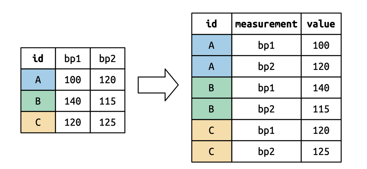
# ℹ 5,297 more rowsdf <- tribble(
~id, ~bp1, ~bp2,
"A", 100, 120,
"B", 140, 115,
"C", 120, 125
)
df# A tibble: 3 × 3
id bp1 bp2
<chr> <dbl> <dbl>
1 A 100 120
2 B 140 115
3 C 120 125df |>
pivot_longer(
    cols = bp1:bp2,
    names_to = "measurement",
    values_to = "value"
)# A tibble: 6 × 3
id measurement value
<chr> <chr> <dbl>
1 A bp1 100
2 A bp2 120
3 B bp1 140
4 B bp2 115
5 C bp1 120
6 C bp2 125pivot_longer(
cols = bp1:bp2,
names_to = "measurement",
values_to = "value"
)
Sometimes, you need to make your data wider. The pivot_wider() function is used when you have one observation spread across multiple rows.
If your column names contain multiple pieces of information, you can split them into separate variables during the pivot process:
who2 |>
  pivot_longer(
    cols = !(country:year),
    names_to = c("diagnosis", "gender", "age"),
    names_sep = "_",
    values_to = "count"
  )
# A tibble: 405,440 × 6
country year diagnosis gender age count
<chr> <dbl> <chr> <chr> <chr> <dbl>
1 Afghanistan 1980 sp m 014 NA
2 Afghanistan 1980 sp m 1524 NA
3 Afghanistan 1980 sp m 2534 NA
4 Afghanistan 1980 sp m 3544 NA
5 Afghanistan 1980 sp m 4554 NA
6 Afghanistan 1980 sp m 5564 NA
7 Afghanistan 1980 sp m 65 NA
8 Afghanistan 1980 sp f 014 NA
9 Afghanistan 1980 sp f 1524 NA
10 Afghanistan 1980 sp f 2534 NA
# ℹ 405,430 more rowsIf a dataset has both variable names and values in its columns, you can use .value in pivot_longer() to separate these:
household |>
  pivot_longer(
    cols = !family,
    names_to = c(".value", "child"),
    names_sep = "_",
    values_drop_na = TRUE
  )
# A tibble: 9 × 4
family child dob name
<int> <chr> <date> <chr>
1 1 child1 1998-11-26 Susan
2 1 child2 2000-01-29 Jose
3 2 child1 1996-06-22 Mark
4 3 child1 2002-07-11 Sam
5 3 child2 2004-04-05 Seth
6 4 child1 2004-10-10 Craig
7 4 child2 2009-08-27 Khai
8 5 child1 2000-12-05 Parker
9 5 child2 2005-02-28 GracieIn this chapter, you’ve learned how to transform your data into a tidy format using pivot_longer() and pivot_wider(). These tools are fundamental for cleaning messy data and making it ready for analysis.
Imagine you have a dataset that tracks the number of visitors to a museum for each day of the week. The data is stored in wide format, where each day of the week is a separate column:
visitors_wide <- tibble(
  museum = c("Museum A", "Museum B", "Museum C"),
  monday = c(120, 150, 110),
  tuesday = c(130, 160, 120),
  wednesday = c(140, 170, 130),
  thursday = c(110, 140, 100),
  friday = c(160, 180, 150)
)
visitors_wide
# A tibble: 3 × 6
museum monday tuesday wednesday thursday friday
<chr> <dbl> <dbl> <dbl> <dbl> <dbl>
1 Museum A 120 130 140 110 160
2 Museum B 150 160 170 140 180
3 Museum C 110 120 130 100 150visitors_long <- visitors_wide |>
pivot_longer(
cols = monday:friday,
names_to = "day",
values_to = "vistors"
)
visitors_long# A tibble: 15 × 3
museum day vistors
<chr> <chr> <dbl>
1 Museum A monday 120
2 Museum A tuesday 130
3 Museum A wednesday 140
4 Museum A thursday 110
5 Museum A friday 160
6 Museum B monday 150
7 Museum B tuesday 160
8 Museum B wednesday 170
9 Museum B thursday 140
10 Museum B friday 180
11 Museum C monday 110
12 Museum C tuesday 120
13 Museum C wednesday 130
14 Museum C thursday 100
15 Museum C friday 150# summary statistics
visitors_long |>
group_by(museum) |>
summarise(
Mean_Num_Vistors = mean(vistors),
Range_Num_Vistors = max(vistors) - min(vistors)
)# A tibble: 3 × 3
museum Mean_Num_Vistors Range_Num_Vistors
<chr> <dbl> <dbl>
1 Museum A 132 50
2 Museum B 160 40
3 Museum C 122 50visitors_long |>
pivot_wider(
names_from = day,
values_from = vistors
)# A tibble: 3 × 6
museum monday tuesday wednesday thursday friday
<chr> <dbl> <dbl> <dbl> <dbl> <dbl>
1 Museum A 120 130 140 110 160
2 Museum B 150 160 170 140 180
3 Museum C 110 120 130 100 150Task 1: Use pivot_longer() to convert this data into a long format where each row represents a single observation of a visitor count for a specific day.
Hint: The names_to argument should be set to “day” to create a column for the days of the week, and the values_to argument should be set to “visitors” to store the number of visitors.
Now, imagine you have a dataset in long format that tracks the average test scores of students in different subjects over several terms. The data is structured like this:
scores_long <- tibble(
  student = c("Alice", "Alice", "Bob", "Bob", "Charlie", "Charlie"),
  term = c("Term 1", "Term 2", "Term 1", "Term 2", "Term 1", "Term 2"),
  subject = c("Math", "Math", "Math", "Math", "Math", "Math"),
  score = c(85, 90, 78, 80, 92, 95)
)
scores_long
# A tibble: 6 × 4
student term subject score
<chr> <chr> <chr> <dbl>
1 Alice Term 1 Math 85
2 Alice Term 2 Math 90
3 Bob Term 1 Math 78
4 Bob Term 2 Math 80
5 Charlie Term 1 Math 92
6 Charlie Term 2 Math 95Task 2: Use pivot_wider() to convert this data into a wide format, where each term is a separate column, and the values represent the student scores.
Hint: The names_from argument should be set to “term” to create columns for each term, and the values_from argument should be set to “score” to get the student scores.
Imagine you have a dataset that tracks the number of calls received by a customer service center over three months for various departments. The dataset is in wide format like this:
calls_wide <- tibble(
  department = c("Sales", "Support", "Billing"),
  jan = c(200, 150, 180),
  feb = c(210, 160, 190),
  mar = c(220, 170, 200)
)
calls_wide
# A tibble: 3 × 4
department jan feb mar
<chr> <dbl> <dbl> <dbl>
1 Sales 200 210 220
2 Support 150 160 170
3 Billing 180 190 200Task 3:
First, use pivot_longer() to convert this dataset into a long format.
Then, use pivot_wider() to convert the data back into a wide format, but with the months as columns and the number of calls as the values.
Now that you understand data tidying, you can begin organizing your analysis in R scripts. In the next chapter, we’ll explore how to use projects and organize your code into files and directories.