0.1 Overview

String and Text Data
Basic Data Summary Using dplyr
Case Study of Trump Tweets
AI + Text Analysis?

1 String and Text Data

1.1 Special Characters

Strings (character-type variable) can be enclosed in either single or double quotes.
```
class("some text")
```
```
[1] "character"
```

If using both within a string, escape necessary quotes using \.

cat("I'm a student")

I'm a student

cat('He says "it is ok!"')

He says "it is ok!"

cat("I'm a student. He says \"it is ok\"!")

I'm a student. He says "it is ok"!

Tip

cat(): Prints the string output directly and escape special symbols.

Use \ to escape special characters such as \n (new line) and \t (tab).

cat("To show \\ , we need to use two of them.")

To show \ , we need to use two of them.

cat("You are my student\nI am your teacher/")

You are my student
I am your teacher/

1.2 Unicode and Other Special Characters

\n and \t: Represent new line and tab space.
\u followed by Unicode code points allows special character insertion.
This Unicode Website can copy and paste freely

test <- "This is the first line. \nThis the \t second line with a tab."
cat(test)

This is the first line. 
This the     second line with a tab.

cat("\u03BC \u03A3 \u03B1 \u03B2")

μ Σ α β

cat("❤ ♫ ⦿")

❤ ♫ ⦿

1.3 Basic String Operations

library(tidyverse)  # Or use stringr: install.packages("stringr")

1.3.1 Creating and Manipulating Strings

tweet1 <- "MAKE AMERICA GREAT AGAIN!"
tweet2 <- "Congratulations @ClemsonFB! https://t.co/w8viax0OWY"

(tweet <- c(tweet1, tweet2))

[1] "MAKE AMERICA GREAT AGAIN!"                          
[2] "Congratulations @ClemsonFB! https://t.co/w8viax0OWY"

Change Case

tolower(tweet)

[1] "make america great again!"                          
[2] "congratulations @clemsonfb! https://t.co/w8viax0owy"

toupper(tweet)

[1] "MAKE AMERICA GREAT AGAIN!"                          
[2] "CONGRATULATIONS @CLEMSONFB! HTTPS://T.CO/W8VIAX0OWY"

Calculate String Length

nchar(tweet1)

[1] 25

str_length(tweet)  # `stringr` alternative

[1] 25 51

1.3.2 Splitting and Combining Strings

Splitting Strings by Pattern

str_split(tweet, pattern = " ")

[[1]]
[1] "MAKE"    "AMERICA" "GREAT"   "AGAIN!" 

[[2]]
[1] "Congratulations"         "@ClemsonFB!"            
[3] "https://t.co/w8viax0OWY"

str_split_1(tweet2, pattern = " https://")  # Returns a vector instead of a list

[1] "Congratulations @ClemsonFB!" "t.co/w8viax0OWY"

Combining Strings

tweet.words <- unlist(str_split(tweet, pattern = " "))
str_c(tweet.words, collapse=" ")

[1] "MAKE AMERICA GREAT AGAIN! Congratulations @ClemsonFB! https://t.co/w8viax0OWY"

2 Data Transformation

2.1 Overview

Data often needs transformation to fit the desired analysis or visualization.
Learn to use the dplyr package for data transformation.
Explore the nycflights13 dataset.

Required Libraries

library(nycflights13) # `nycflights13` for the dataset flights.
library(tidyverse)
glimpse(flights)

Rows: 336,776
Columns: 19
$ year           <int> 2013, 2013, 2013, 2013, 2013, 2013, 2013, 2013, 2013, 2…
$ month          <int> 1, 1, 1, 1, 1, 1, 1, 1, 1, 1, 1, 1, 1, 1, 1, 1, 1, 1, 1…
$ day            <int> 1, 1, 1, 1, 1, 1, 1, 1, 1, 1, 1, 1, 1, 1, 1, 1, 1, 1, 1…
$ dep_time       <int> 517, 533, 542, 544, 554, 554, 555, 557, 557, 558, 558, …
$ sched_dep_time <int> 515, 529, 540, 545, 600, 558, 600, 600, 600, 600, 600, …
$ dep_delay      <dbl> 2, 4, 2, -1, -6, -4, -5, -3, -3, -2, -2, -2, -2, -2, -1…
$ arr_time       <int> 830, 850, 923, 1004, 812, 740, 913, 709, 838, 753, 849,…
$ sched_arr_time <int> 819, 830, 850, 1022, 837, 728, 854, 723, 846, 745, 851,…
$ arr_delay      <dbl> 11, 20, 33, -18, -25, 12, 19, -14, -8, 8, -2, -3, 7, -1…
$ carrier        <chr> "UA", "UA", "AA", "B6", "DL", "UA", "B6", "EV", "B6", "…
$ flight         <int> 1545, 1714, 1141, 725, 461, 1696, 507, 5708, 79, 301, 4…
$ tailnum        <chr> "N14228", "N24211", "N619AA", "N804JB", "N668DN", "N394…
$ origin         <chr> "EWR", "LGA", "JFK", "JFK", "LGA", "EWR", "EWR", "LGA",…
$ dest           <chr> "IAH", "IAH", "MIA", "BQN", "ATL", "ORD", "FLL", "IAD",…
$ air_time       <dbl> 227, 227, 160, 183, 116, 150, 158, 53, 140, 138, 149, 1…
$ distance       <dbl> 1400, 1416, 1089, 1576, 762, 719, 1065, 229, 944, 733, …
$ hour           <dbl> 5, 5, 5, 5, 6, 5, 6, 6, 6, 6, 6, 6, 6, 6, 6, 5, 6, 6, 6…
$ minute         <dbl> 15, 29, 40, 45, 0, 58, 0, 0, 0, 0, 0, 0, 0, 0, 0, 59, 0…
$ time_hour      <dttm> 2013-01-01 05:00:00, 2013-01-01 05:00:00, 2013-01-01 0…

glimpse() for the quick screening of the data.

2.2 `dplyr` Core Functions

filter(): Subset rows based on conditions.
arrange(): Reorder rows.
select(): Choose columns by name.
mutate(): Create new columns.
summarize(): Aggregate data.
group_by(): group data for summarization.

Operators

All following operators will return TRUE or FALSE:
- Comparison operators: ==, !=, <, <=, >, >=.
- Logical operators: &, |, !.
- Inclusion operator: %in%, i.e., 3 %in% c(1,2,3) will return TRUE
```
flights |> filter(month != 1) # Months other than January
flights |> filter(month %in% 1:10) # Months other than Nov. and Dec.
```

2.2.1 `filter()`: select cases based on condtions

Use |> (Preferred, a vertical line symbol | plus a greater symbol >) or %>% to chain multiple functions/operations (shortcut: ).

Aim: Select flights on January 1st:

Compare whether month,day equal to “1” (Januarary) and “1” (1^st day), respectively

jan1 <- flights |> filter(month == 1, day == 1)
jan1

# A tibble: 842 × 19
    year month   day dep_time sched_dep_time dep_delay arr_time sched_arr_time
   <int> <int> <int>    <int>          <int>     <dbl>    <int>          <int>
 1  2013     1     1      517            515         2      830            819
 2  2013     1     1      533            529         4      850            830
 3  2013     1     1      542            540         2      923            850
 4  2013     1     1      544            545        -1     1004           1022
 5  2013     1     1      554            600        -6      812            837
 6  2013     1     1      554            558        -4      740            728
 7  2013     1     1      555            600        -5      913            854
 8  2013     1     1      557            600        -3      709            723
 9  2013     1     1      557            600        -3      838            846
10  2013     1     1      558            600        -2      753            745
# ℹ 832 more rows
# ℹ 11 more variables: arr_delay <dbl>, carrier <chr>, flight <int>,
#   tailnum <chr>, origin <chr>, dest <chr>, air_time <dbl>, distance <dbl>,
#   hour <dbl>, minute <dbl>, time_hour <dttm>

2.2.2 `arrange()`: Arranging Rows

Sort flights by departure delay:

flights[, c("year", "month", "day", "dep_delay")] |> arrange(dep_delay)

# A tibble: 336,776 × 4
    year month   day dep_delay
   <int> <int> <int>     <dbl>
 1  2013    12     7       -43
 2  2013     2     3       -33
 3  2013    11    10       -32
 4  2013     1    11       -30
 5  2013     1    29       -27
 6  2013     8     9       -26
 7  2013    10    23       -25
 8  2013     3    30       -25
 9  2013     3     2       -24
10  2013     5     5       -24
# ℹ 336,766 more rows

Descending order:

flights[, c("year", "month", "day", "dep_delay")] |> arrange(desc(dep_delay))

# A tibble: 336,776 × 4
    year month   day dep_delay
   <int> <int> <int>     <dbl>
 1  2013     1     9      1301
 2  2013     6    15      1137
 3  2013     1    10      1126
 4  2013     9    20      1014
 5  2013     7    22      1005
 6  2013     4    10       960
 7  2013     3    17       911
 8  2013     6    27       899
 9  2013     7    22       898
10  2013    12     5       896
# ℹ 336,766 more rows

2.2.3 `select()`: Selecting Columns

Choose specific columns:

flights |> select(year, month, day)

# A tibble: 336,776 × 3
    year month   day
   <int> <int> <int>
 1  2013     1     1
 2  2013     1     1
 3  2013     1     1
 4  2013     1     1
 5  2013     1     1
 6  2013     1     1
 7  2013     1     1
 8  2013     1     1
 9  2013     1     1
10  2013     1     1
# ℹ 336,766 more rows

## is equivalent to 
# flights[, c("year", "month", "day")]

Helper functions for selecting the variables: starts_with(), ends_with(), contains(), matches(), num_range().

2.2.4 `mutate()`: Adding New Variables

Create new columns:

flights_sml <- flights |> select(
  year:day,
  ends_with("delay"),
  distance,
  air_time
)

flights_sml |> mutate(
  gain = dep_delay - arr_delay,
  speed = distance / air_time * 60
) |> 
  select(year:day, gain, speed)

# A tibble: 336,776 × 5
    year month   day  gain speed
   <int> <int> <int> <dbl> <dbl>
 1  2013     1     1    -9  370.
 2  2013     1     1   -16  374.
 3  2013     1     1   -31  408.
 4  2013     1     1    17  517.
 5  2013     1     1    19  394.
 6  2013     1     1   -16  288.
 7  2013     1     1   -24  404.
 8  2013     1     1    11  259.
 9  2013     1     1     5  405.
10  2013     1     1   -10  319.
# ℹ 336,766 more rows

Use transmute() to keep only the new variables.

flights_sml |> transmute(
  gain = dep_delay - arr_delay,
  speed = distance / air_time * 60
)

# A tibble: 336,776 × 2
    gain speed
   <dbl> <dbl>
 1    -9  370.
 2   -16  374.
 3   -31  408.
 4    17  517.
 5    19  394.
 6   -16  288.
 7   -24  404.
 8    11  259.
 9     5  405.
10   -10  319.
# ℹ 336,766 more rows

`mutate()` and `case_when`: Create new categories

case_when: The left hand side (LHS) determines which values match this case. The right hand side (RHS) provides the replacement value.
- The LHS inputs must evaluate to logical vectors.
- The RHS inputs will be coerced to their common type. In following case, it is character type

x <- c(1:10, NA)
categorized_x <- case_when(
  x %in% 1:3 ~ "low",
  x %in% 4:7 ~ "med",
  x %in% 7:10 ~ "high",
  is.na(x) ~ "Missing"
)
categorized_x

 [1] "low"     "low"     "low"     "med"     "med"     "med"     "med"    
 [8] "high"    "high"    "high"    "Missing"

Combine mutate() and case_when() to create a new categorical variable
- na.rm = TRUE to ignore the NA values when calculating the mean

flights |> 
  mutate(
    Half_year = case_when(
      month %in% 1:6 ~ 1,
      month %in% 6:12 ~ 2,
      is.na(month) ~ 999
    )
  ) |> 
  group_by(year, Half_year) |> 
  summarise(
    Mean_dep_delay = mean(dep_delay, na.rm = TRUE)
  )

# A tibble: 2 × 3
# Groups:   year [1]
   year Half_year Mean_dep_delay
  <int>     <dbl>          <dbl>
1  2013         1           13.7
2  2013         2           11.6

2.2.5 `summarize()` with `group_by()`: Summarizing Data

Calculate average delay by destination:

by_dest <- flights |> group_by(dest)
delay <- summarize(by_dest,
  count = n(),
  dist = mean(distance, na.rm = TRUE),
  delay = mean(arr_delay, na.rm = TRUE)
)

Visualize the results:

ggplot(data = delay, mapping = aes(x = dist, y = delay)) +
  geom_point(aes(size = count), alpha = 1/3) +
  geom_smooth(se = FALSE)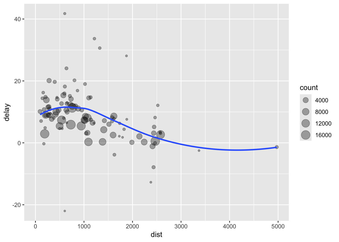

2.2.6 `group_by()` and `ungroup()`: Grouping and Ungrouping

Group data by multiple variables:

by_day <- flights |> group_by(year, month, day)
by_day |> 
  summarize(avg_dep_delay = mean(dep_delay, na.rm = TRUE))

# A tibble: 365 × 4
# Groups:   year, month [12]
    year month   day avg_dep_delay
   <int> <int> <int>         <dbl>
 1  2013     1     1         11.5 
 2  2013     1     2         13.9 
 3  2013     1     3         11.0 
 4  2013     1     4          8.95
 5  2013     1     5          5.73
 6  2013     1     6          7.15
 7  2013     1     7          5.42
 8  2013     1     8          2.55
 9  2013     1     9          2.28
10  2013     1    10          2.84
# ℹ 355 more rows

Ungroup data:

by_day <- ungroup(by_day)

2.3 More dplyr Functions

rename(): Renaming Columns.
relocate(): Reorder column position.
distinct(): Choose distinct/unique cases.
count(): Create group size.
slice(): Select cases or random sampling.
rowwise(): Perform calculations for each row.

2.3.1 `rename()`: Renaming Columns

# Rename columns
df <- flights |> rename(
  departure_time = dep_time,
  arrival_time = arr_time,
  departure_delay = dep_delay,
  arrival_delay = arr_delay
)
glimpse(df)

Rows: 336,776
Columns: 19
$ year            <int> 2013, 2013, 2013, 2013, 2013, 2013, 2013, 2013, 2013, …
$ month           <int> 1, 1, 1, 1, 1, 1, 1, 1, 1, 1, 1, 1, 1, 1, 1, 1, 1, 1, …
$ day             <int> 1, 1, 1, 1, 1, 1, 1, 1, 1, 1, 1, 1, 1, 1, 1, 1, 1, 1, …
$ departure_time  <int> 517, 533, 542, 544, 554, 554, 555, 557, 557, 558, 558,…
$ sched_dep_time  <int> 515, 529, 540, 545, 600, 558, 600, 600, 600, 600, 600,…
$ departure_delay <dbl> 2, 4, 2, -1, -6, -4, -5, -3, -3, -2, -2, -2, -2, -2, -…
$ arrival_time    <int> 830, 850, 923, 1004, 812, 740, 913, 709, 838, 753, 849…
$ sched_arr_time  <int> 819, 830, 850, 1022, 837, 728, 854, 723, 846, 745, 851…
$ arrival_delay   <dbl> 11, 20, 33, -18, -25, 12, 19, -14, -8, 8, -2, -3, 7, -…
$ carrier         <chr> "UA", "UA", "AA", "B6", "DL", "UA", "B6", "EV", "B6", …
$ flight          <int> 1545, 1714, 1141, 725, 461, 1696, 507, 5708, 79, 301, …
$ tailnum         <chr> "N14228", "N24211", "N619AA", "N804JB", "N668DN", "N39…
$ origin          <chr> "EWR", "LGA", "JFK", "JFK", "LGA", "EWR", "EWR", "LGA"…
$ dest            <chr> "IAH", "IAH", "MIA", "BQN", "ATL", "ORD", "FLL", "IAD"…
$ air_time        <dbl> 227, 227, 160, 183, 116, 150, 158, 53, 140, 138, 149, …
$ distance        <dbl> 1400, 1416, 1089, 1576, 762, 719, 1065, 229, 944, 733,…
$ hour            <dbl> 5, 5, 5, 5, 6, 5, 6, 6, 6, 6, 6, 6, 6, 6, 6, 5, 6, 6, …
$ minute          <dbl> 15, 29, 40, 45, 0, 58, 0, 0, 0, 0, 0, 0, 0, 0, 0, 59, …
$ time_hour       <dttm> 2013-01-01 05:00:00, 2013-01-01 05:00:00, 2013-01-01 …

2.3.2 `relocate()`: Changing Column Order

# Move the "year" column after "carrier" column
df |> 
  select(carrier, departure_time, arrival_time, year) |> 
  relocate(year, .after = carrier)

# A tibble: 336,776 × 4
   carrier  year departure_time arrival_time
   <chr>   <int>          <int>        <int>
 1 UA       2013            517          830
 2 UA       2013            533          850
 3 AA       2013            542          923
 4 B6       2013            544         1004
 5 DL       2013            554          812
 6 UA       2013            554          740
 7 B6       2013            555          913
 8 EV       2013            557          709
 9 B6       2013            557          838
10 AA       2013            558          753
# ℹ 336,766 more rows

2.3.3 `distinct()`: Remove Duplicates

unique() function outputs unique values from a vector.
distinct() function outputs unique cases from a dataset

unique(c(1, 2, 3, 4, 4, 5, 5))

[1] 1 2 3 4 5

# flights with unique carrier-destination pairs
df |> 
  distinct(carrier, dest)

# A tibble: 314 × 2
   carrier dest 
   <chr>   <chr>
 1 UA      IAH  
 2 AA      MIA  
 3 B6      BQN  
 4 DL      ATL  
 5 UA      ORD  
 6 B6      FLL  
 7 EV      IAD  
 8 B6      MCO  
 9 AA      ORD  
10 B6      PBI  
# ℹ 304 more rows

2.3.4 `count()`: Quick Grouping & Summarization

# Count number of flights per carrier
df |> count(carrier, sort = TRUE)

# A tibble: 16 × 2
   carrier     n
   <chr>   <int>
 1 UA      58665
 2 B6      54635
 3 EV      54173
 4 DL      48110
 5 AA      32729
 6 MQ      26397
 7 US      20536
 8 9E      18460
 9 WN      12275
10 VX       5162
11 FL       3260
12 AS        714
13 F9        685
14 YV        601
15 HA        342
16 OO         32

# equivalent to
if (0) {
df |> 
  group_by(carrier) |> 
  summarise(
    n = n()
  )
}

2.3.5 `slice()`: Selecting Specific Rows

slice_*() family allows you to choose rows based on their positions

# Select the first 10 flights
df |> slice(1:10)

# A tibble: 10 × 19
    year month   day departure_time sched_dep_time departure_delay arrival_time
   <int> <int> <int>          <int>          <int>           <dbl>        <int>
 1  2013     1     1            517            515               2          830
 2  2013     1     1            533            529               4          850
 3  2013     1     1            542            540               2          923
 4  2013     1     1            544            545              -1         1004
 5  2013     1     1            554            600              -6          812
 6  2013     1     1            554            558              -4          740
 7  2013     1     1            555            600              -5          913
 8  2013     1     1            557            600              -3          709
 9  2013     1     1            557            600              -3          838
10  2013     1     1            558            600              -2          753
# ℹ 12 more variables: sched_arr_time <int>, arrival_delay <dbl>,
#   carrier <chr>, flight <int>, tailnum <chr>, origin <chr>, dest <chr>,
#   air_time <dbl>, distance <dbl>, hour <dbl>, minute <dbl>, time_hour <dttm>

# Select the top 5 flights with the highest departure delay
df |> slice_max(departure_delay, n = 5)

# A tibble: 5 × 19
   year month   day departure_time sched_dep_time departure_delay arrival_time
  <int> <int> <int>          <int>          <int>           <dbl>        <int>
1  2013     1     9            641            900            1301         1242
2  2013     6    15           1432           1935            1137         1607
3  2013     1    10           1121           1635            1126         1239
4  2013     9    20           1139           1845            1014         1457
5  2013     7    22            845           1600            1005         1044
# ℹ 12 more variables: sched_arr_time <int>, arrival_delay <dbl>,
#   carrier <chr>, flight <int>, tailnum <chr>, origin <chr>, dest <chr>,
#   air_time <dbl>, distance <dbl>, hour <dbl>, minute <dbl>, time_hour <dttm>

# Select the 5 flights with the lowest arrival delay
df |> slice_min(arrival_delay, n = 5)

# A tibble: 5 × 19
   year month   day departure_time sched_dep_time departure_delay arrival_time
  <int> <int> <int>          <int>          <int>           <dbl>        <int>
1  2013     5     7           1715           1729             -14         1944
2  2013     5    20            719            735             -16          951
3  2013     5     2           1947           1949              -2         2209
4  2013     5     6           1826           1830              -4         2045
5  2013     5     4           1816           1820              -4         2017
# ℹ 12 more variables: sched_arr_time <int>, arrival_delay <dbl>,
#   carrier <chr>, flight <int>, tailnum <chr>, origin <chr>, dest <chr>,
#   air_time <dbl>, distance <dbl>, hour <dbl>, minute <dbl>, time_hour <dttm>

2.3.6 `slice_sample()`: Random Sampling

# Randomly select 5 flights
df |> slice_sample(n = 5)

# A tibble: 5 × 19
   year month   day departure_time sched_dep_time departure_delay arrival_time
  <int> <int> <int>          <int>          <int>           <dbl>        <int>
1  2013    12     5           1029           1030              -1         1418
2  2013    11    20           1907           1910              -3         2225
3  2013     9    18           1009           1015              -6         1201
4  2013     7    31           1458           1459              -1         1819
5  2013    12    11            746            748              -2         1059
# ℹ 12 more variables: sched_arr_time <int>, arrival_delay <dbl>,
#   carrier <chr>, flight <int>, tailnum <chr>, origin <chr>, dest <chr>,
#   air_time <dbl>, distance <dbl>, hour <dbl>, minute <dbl>, time_hour <dttm>

# Select 1% random sample
df |> slice_sample(prop = 0.01)

# A tibble: 3,367 × 19
    year month   day departure_time sched_dep_time departure_delay arrival_time
   <int> <int> <int>          <int>          <int>           <dbl>        <int>
 1  2013    11     1           2055           2100              -5         2349
 2  2013    11     4           1926           1930              -4         2147
 3  2013    10     9           2146           2100              46           17
 4  2013    12    12           1630           1620              10         1923
 5  2013     9    29           1643           1630              13         1939
 6  2013     1    16           1239           1240              -1         1450
 7  2013     4     2           1653           1700              -7         1819
 8  2013     7    26            630            630               0          824
 9  2013     7     9           1449           1455              -6         1644
10  2013     6     4           1949           1955              -6         2110
# ℹ 3,357 more rows
# ℹ 12 more variables: sched_arr_time <int>, arrival_delay <dbl>,
#   carrier <chr>, flight <int>, tailnum <chr>, origin <chr>, dest <chr>,
#   air_time <dbl>, distance <dbl>, hour <dbl>, minute <dbl>, time_hour <dttm>

2.3.7 `rowwise()`: Row-Wise Grouping Operations

Similar to group_by, but each row/case will be considered as one group
When you’re working with a rowwise tibble, then dplyr will use [[ instead of [ to make your life a little easier.
Assume you want to calculate the mean of variables x, y and c: $\frac{x + y + z}{3}$

set.seed(1234)
xyz <- tibble(x = runif(6), y = runif(6), z = runif(6))
rowMeans(xyz[, c("x", "y", "z")])

[1] 0.1353109 0.5927611 0.5225581 0.6583087 0.6135767 0.4840354

# Compute the mean of x, y, z in each row
xyz |> 
  rowwise() |> 
  mutate(m = mean(c(x, y, z)))

# A tibble: 6 × 4
# Rowwise: 
      x       y     z     m
  <dbl>   <dbl> <dbl> <dbl>
1 0.114 0.00950 0.283 0.135
2 0.622 0.233   0.923 0.593
3 0.609 0.666   0.292 0.523
4 0.623 0.514   0.837 0.658
5 0.861 0.694   0.286 0.614
6 0.640 0.545   0.267 0.484

# Compute the total delay per flight
df |> 
  rowwise() |> 
  mutate(avg_delay_time_perMile = sum(departure_delay, arrival_delay, na.rm = TRUE) / distance,
         .keep = "used")

# A tibble: 336,776 × 4
# Rowwise: 
   departure_delay arrival_delay distance avg_delay_time_perMile
             <dbl>         <dbl>    <dbl>                  <dbl>
 1               2            11     1400                0.00929
 2               4            20     1416                0.0169 
 3               2            33     1089                0.0321 
 4              -1           -18     1576               -0.0121 
 5              -6           -25      762               -0.0407 
 6              -4            12      719                0.0111 
 7              -5            19     1065                0.0131 
 8              -3           -14      229               -0.0742 
 9              -3            -8      944               -0.0117 
10              -2             8      733                0.00819
# ℹ 336,766 more rows

Tip

.keep = "used" retains only the columns used in ... to create new columns. This is useful for checking your work, as it displays inputs and outputs side-by-side.

2.4 Summary & Takeaways

dplyr provides powerful tools for data transformation.
Combining functions allows for efficient data manipulation.
group_by() and summarize() are key for data aggregation.
Functions like rename(), slice(), relocate(), and case_when() enhance usability.

3 Motivating Example: AI + Text Analysis

3.1 Extract Structural Information from Text

Make use of language models to extract key information from a unstructral text file
This is not a step-by-step guide of using LLMs, but a motivating example so that you may want to explore more usage of LLMs in data analysis.
- The details of techniques can be found in this link.
Note that the following code cannot be successfully executed in your local device without ChatGPT account and access to API keys.
- Here is a video tutorial for using ChatGPT in R.

3.2 Programming LLMs in R

Rather than using ChatBot on the OpenAI website, to programming LLMs for text analysis, I suggested using ellmer package (the manual) which was developed by the same person who developed tidyverse package.

library(ellmer)
chat <- chat_openai(echo = FALSE, model = "gpt-4o-mini")

chat$extract_data(
  tweet2,
  type = type_object(
    URL = type_string("URL address starting with 'http'")
  )  
)

$URL
[1] "https://t.co/w8viax0OWY"

chat$extract_data(
  "My name is Susan and I'm 13 years old. I like traveling and hiking.",
  type = type_object(
    age = type_number("Age, in years."), # extract the numeric information as "age" from the provided text
    name = type_string("Name, Uppercase"), # extract the character information as "name" from the provided text
    hobbies = type_array(
      description = "List of hobbies. Uppercase",
      items = type_string()
    )
  )
)

$age
[1] 13

$name
[1] "SUSAN"

$hobbies
[1] "TRAVELING" "HIKING"

Here, type_*() specify object types in a way that LLMs can understand and are used for structured data extraction.

3.3 Article Summarisation

library(pdftools)
paper_text <- paste0(pdf_text("example_paper.pdf"), collapse = "\n")

type_summary <- type_object(
  "Summary of the article.",
  author = type_string("Name of the article author"),
  topics = type_array(
    'Array of topics, e.g. ["tech", "politics"]. Should be as specific as possible, and can overlap.',
    type_string(),
  ),
  design = type_string("Summary of research design of the article. One or two paragraphs max"),
  measures = type_string("Key indices in results"),
  finding = type_string("Summary of key findings. One paragraph max")
)

chat <- chat_openai(model = "gpt-4o-mini")
data <- chat$extract_data(paper_text, type = type_summary)
str(data)

List of 5
 $ author  : chr "Yunting Liu, Shreya Bhandari, Zachary A. Pardos"
 $ topics  : chr [1:4] "Large Language Models" "Psychometric Analysis" "Educational Measurement" "Item Response Theory"
 $ design  : chr "This study investigates the ability of various Large Language Models (LLMs) to produce responses to College Alg"| __truncated__
 $ measures: chr "Key indices include Pearson and Spearman correlation coefficients comparing item parameters calibrated from AI "| __truncated__
 $ finding : chr "The findings demonstrate that while certain LLMs, particularly GPT-3.5 and GPT-4, can achieve performance level"| __truncated__

cat(data$author)

Yunting Liu, Shreya Bhandari, Zachary A. Pardos

print(data$topics)

[1] "Large Language Models"   "Psychometric Analysis"  
[3] "Educational Measurement" "Item Response Theory"

print(data$design)

[1] "This study investigates the ability of various Large Language Models (LLMs) to produce responses to College Algebra assessment items that are psychometrically similar to human responses. Six models (GPT-3.5, GPT-4, Llama 2, Llama 3, Gemini-Pro, and Cohere Command R Plus) were utilized to generate responses based on items sourced from an OpenStax textbook. A total of 150 responses were generated per model and compared against a human response set obtained from undergraduate students. Item Response Theory (IRT) was employed to compare the psychometric properties of these AI-generated responses to those from human participants. Data augmentation strategies were tested to enhance item parameter calibration by combining human and AI-generated responses."

print(data$measures)

[1] "Key indices include Pearson and Spearman correlation coefficients comparing item parameters calibrated from AI responses to those derived from human responses, with results showing Spearman correlations as high as 0.93 in augmented scenarios."

print(data$finding)

[1] "The findings demonstrate that while certain LLMs, particularly GPT-3.5 and GPT-4, can achieve performance levels comparable to or exceeding average college students in College Algebra, they do not sufficiently replicate the variability of human responses. The most effective augmentation strategy combined human responses with a 1:1 ratio of resampled LLM responses, yielding improvements in correlation metrics. Although reliance solely on LLMs is inadequate for simulating human response variability, their integration offers a cost-effective means for educational measurement item calibration."

3.4 Open Sourced Local Distilled Models

You can freely download the open source LLM - Llama developed by Meta on this link.
Teaching how to set up the LLMs is out of scope of this class. There are a lot of tutorials that you can use. For example, this medium post.
Just showcase how you can extract key information. Llama needs more guide information to extract certain key words than ChatGPT.

chat <- chat_ollama(model = "llama3.2")

chat$extract_data(
  "My name is Jihong and I'm an assistant professor. I like reading and hiking.",
  type = type_object(
    job = type_string("Job"), # extract the numeric information as "age" from the provided text
    name = type_string("Name of the person, uppercase"), # extract the character information as "name" from the provided text
    hobbies = type_array(
      description = "List of hobbies. transform to Uppercase",
      items = type_string()
    )
  )
)

$job
[1] "assistant professor"

$name
[1] "Jihong"

$hobbies
[1] "reading" "hiking"

3.4.1 Deepseek distilled model

chat <- chat_ollama(model = "deepseek-r1:8b")

Text_to_summarize <- "Results of Paper: Researchers have devised an ecological momentary assessment study following 80 students (mean age = 20.38 years, standard deviation = 3.68, range = 18–48 years; n = 60 female, n = 19 male, n = 1 other) from Leiden University for 2 weeks in their daily lives."

type_summarize_results = type_object(
    N = type_number("Total sample size the study used"),
    Age = type_number("Average age in years"),
    Method = type_string("Assessment for data collection"),
    Participants = type_string("source of data collection"),
    Days = type_string("Duration of data collection")
)
chat$extract_data(
  Text_to_summarize,
  type = type_summarize_results
)

$N
[1] 40

$Age
[1] 20.38

$Method
[1] "Ecological momentary assessment study"

$Participants
[1] "n=40 students"

$Days
[1] "2 weeks"

4 Case Study: Analysis of Trump Tweets

4.1 Download of Trump Tweets

For demonstration, we will analyze the tweets from President Donald Trump from 2009 to 2017.

library(dslabs) # install.packages("dslabs")
library(tidyverse) 
glimpse(dslabs::trump_tweets)

Rows: 20,761
Columns: 8
$ source                  <chr> "Twitter Web Client", "Twitter Web Client", "T…
$ id_str                  <chr> "6971079756", "6312794445", "6090839867", "577…
$ text                    <chr> "From Donald Trump: Wishing everyone a wonderf…
$ created_at              <dttm> 2009-12-23 12:38:18, 2009-12-03 14:39:09, 200…
$ retweet_count           <int> 28, 33, 13, 5, 7, 4, 2, 4, 1, 22, 7, 5, 1, 1, …
$ in_reply_to_user_id_str <chr> NA, NA, NA, NA, NA, NA, NA, NA, NA, NA, NA, NA…
$ favorite_count          <int> 12, 6, 11, 3, 6, 5, 2, 10, 4, 30, 6, 3, 4, 3, …
$ is_retweet              <lgl> FALSE, FALSE, FALSE, FALSE, FALSE, FALSE, FALS…

Note

source. Device or service used to compose tweet.
id_str. Tweet ID.
text. Tweet.
created_at. Data and time tweet was tweeted.
retweet_count. How many times tweet had been retweeted at time dataset was created.
in_reply_to_user_id_str. If a reply, the user id of person being replied to.
favorite_count. Number of times tweet had been favored at time dataset was created.
is_retweet. A logical telling us if it is a retweet or not.

4.2 Basic summary of Trump tweets

Where the tweets were sent from

trump_tweets |> 
  group_by(
    source
  ) |> 
  summarise(N = n()) |> 
  arrange(desc(N))

# A tibble: 19 × 2
   source                       N
   <chr>                    <int>
 1 Twitter Web Client       10718
 2 Twitter for Android       4652
 3 Twitter for iPhone        3962
 4 TweetDeck                  468
 5 TwitLonger Beta            288
 6 Instagram                  133
 7 Media Studio               114
 8 Facebook                   104
 9 Twitter Ads                 96
10 Twitter for BlackBerry      78
11 Mobile Web (M5)             54
12 Twitter for iPad            39
13 Twitlonger                  22
14 Twitter QandA               10
15 Vine - Make a Scene         10
16 Periscope                    7
17 Neatly For BlackBerry 10     4
18 Twitter Mirror for iPad      1
19 Twitter for Websites         1

4.2.1 Histogram of tweet sources

⌘+C

n_source_tbl <- trump_tweets |> 
  group_by(source) |> 
  summarise(
    N = n()
  )
ggplot(data = n_source_tbl) +
  geom_col(aes(x = fct_reorder(source, N), y = N)) +
  geom_label(aes(x = fct_reorder(source, N), y = N, label = N), nudge_y = 500) +
  labs(x = "", y = "") +
  coord_flip()

4.2.2 The length of each tweet

summary(str_length(trump_tweets$text))

   Min. 1st Qu.  Median    Mean 3rd Qu.    Max. 
    2.0    81.0   119.0   106.4   137.0   320.0

Most tweets have the length from 100 to 150 characters.
Filter the tweet less than 20 characters

trump_short_tweets <- trump_tweets |> 
  mutate(
    N_characters = str_length(text)
  ) |> 
  filter(N_characters <= 20)

4.3 Extract Frequent Words from the Short Tweets

trump_short_clean_tweets <- trump_short_tweets |> 
  mutate(
    clean_text = str_remove(text, "@\\S+ ")
  ) |> 
  mutate(
    clean_text2 = str_remove_all(clean_text, "[[:punct:]]") # Remove punctuation
  ) |> 
  select(text, clean_text, clean_text2)
slice_sample(trump_short_clean_tweets, n = 5)

                  text  clean_text clean_text2
1    @maggiedubh  Yes.        Yes.         Yes
2    @jrkirk22 Thanks.     Thanks.      Thanks
3 @tkeller316  Thanks!     Thanks!      Thanks
4      @CRLindke True!       True!        True
5 @Corte74  It helped!  It helped!   It helped

Explanation of the Regular Expression:

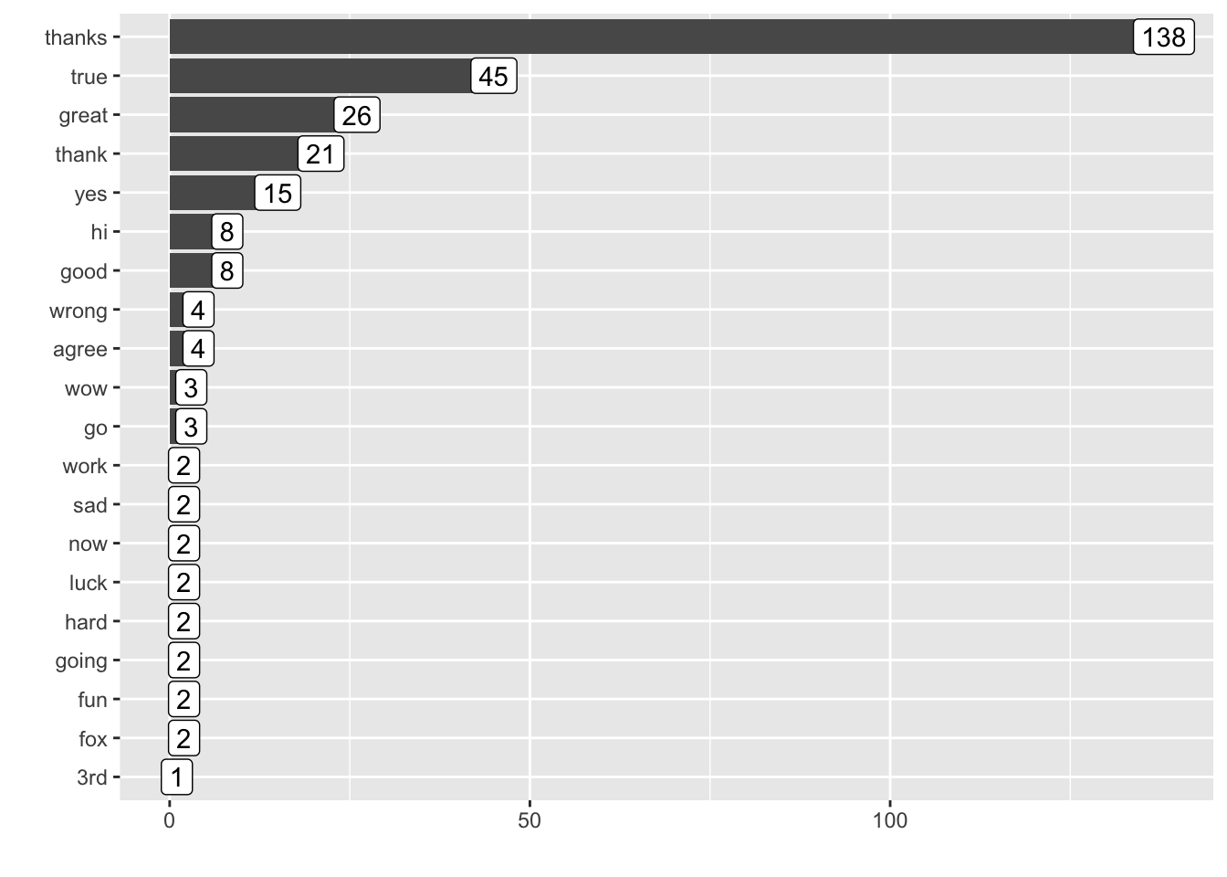
@ matches the @ symbol.
\\S+ matches one or more non-whitespace characters (i.e., the username).
str_remove() removes the matched pattern.

Top 20 most frequently used words

⌘+C

trump.split <- unlist(str_split(trump_short_clean_tweets$clean_text2, 
                                pattern = " "))

word.freq <- as.data.frame(sort(table(word = tolower(trump.split)), decreasing = T))

word_freq_tbl <- word.freq |> 
  mutate(word = trimws(word)) |> 
  filter(
    word != "",
    !(word %in% stopwords::stopwords("en")),
    !(word %in% c("I", "&amp;", "The", "-", "just"))
  )

ggplot(data = word_freq_tbl[1:20, ]) +
  geom_col(aes(x = fct_reorder(word, Freq), y = Freq)) +
  geom_label(aes(x = fct_reorder(word, Freq), y = Freq, label = Freq)) +
  labs(x = "", y = "") +
  coord_flip()

0.1 Overview

1 String and Text Data

1.1 Special Characters

1.2 Unicode and Other Special Characters

1.3 Basic String Operations

1.3.1 Creating and Manipulating Strings

Change Case

Calculate String Length

1.3.2 Splitting and Combining Strings

Splitting Strings by Pattern

Combining Strings

2 Data Transformation

2.1 Overview

2.2 dplyr Core Functions

2.2.1 filter(): select cases based on condtions

2.2.2 arrange(): Arranging Rows

2.2.3 select(): Selecting Columns

2.2.4 mutate(): Adding New Variables

mutate() and case_when: Create new categories

2.2.5 summarize() with group_by(): Summarizing Data

2.2.6 group_by() and ungroup(): Grouping and Ungrouping

2.3 More dplyr Functions

2.3.1 rename(): Renaming Columns

2.3.2 relocate(): Changing Column Order

2.3.3 distinct(): Remove Duplicates

2.3.4 count(): Quick Grouping & Summarization

2.3.5 slice(): Selecting Specific Rows

2.3.6 slice_sample(): Random Sampling

2.3.7 rowwise(): Row-Wise Grouping Operations

2.4 Summary & Takeaways

3 Motivating Example: AI + Text Analysis

3.1 Extract Structural Information from Text

3.2 Programming LLMs in R

3.3 Article Summarisation

3.4 Open Sourced Local Distilled Models

3.4.1 Deepseek distilled model

4 Case Study: Analysis of Trump Tweets

4.1 Download of Trump Tweets

4.2 Basic summary of Trump tweets

4.2.1 Histogram of tweet sources

4.2.2 The length of each tweet

4.3 Extract Frequent Words from the Short Tweets

4.4 Reference

2.2 `dplyr` Core Functions

2.2.1 `filter()`: select cases based on condtions

2.2.2 `arrange()`: Arranging Rows

2.2.3 `select()`: Selecting Columns

2.2.4 `mutate()`: Adding New Variables

`mutate()` and `case_when`: Create new categories

2.2.5 `summarize()` with `group_by()`: Summarizing Data

2.2.6 `group_by()` and `ungroup()`: Grouping and Ungrouping

2.3.1 `rename()`: Renaming Columns

2.3.2 `relocate()`: Changing Column Order

2.3.3 `distinct()`: Remove Duplicates

2.3.4 `count()`: Quick Grouping & Summarization

2.3.5 `slice()`: Selecting Specific Rows

2.3.6 `slice_sample()`: Random Sampling

2.3.7 `rowwise()`: Row-Wise Grouping Operations