Today’s Class

Today's Class

Multivaraite regression via path model
Model modification
Comparing and contrasting path analysis

Differences in model fit measures

How to interpret the results of path model

library(ESRM64503)
library(kableExtra)
library(tidyverse)
library(DescTools) # Desc() allows you to quick screen data
library(lavaan) # Desc() allows you to quick screen data
# options(digits = 3)
head(dataMath)

  id hsl cc use msc mas mse perf female
1  1  NA  9  44  55  39  NA   14      1
2  2   3  2  77  70  42  71   12      0
3  3  NA 12  64  52  31  NA   NA      1
4  4   6 20  71  65  39  84   19      0
5  5   2 15  48  19   2  60   12      0
6  6  NA 15  61  62  42  87   18      0

dim(dataMath)

[1] 350   9

Path Analysis

Previous models considered correlations among observed variables (perf and use). These models may be limited in answering more complex research questions: whether A is a mediator between B and C
Path analysis: Multivariate Linear Models where Outcomes can be also Predictors
Path analysis details:
- Model identification
- Modeling workflow
Example Analyses

Today’s Example Data

Data are simulated based on the results reported in:
Sample of 350 undergraduates (229 women, 121 men)
- In simulation, 10% of variables were missing (using missing completely at random mechanism).

Dictionary

Prior Experience at High School Level (HSL)
Prior Experience at College Level (CC)
Perceived Usefulness of Mathematics (USE)
Math Self-Concept (MSC)
Math Anxiety (MAS)
Math Self-Efficacy (MSE)
Math Performance (PERF)
Female (sex variable: 0 = male; 1 = female)

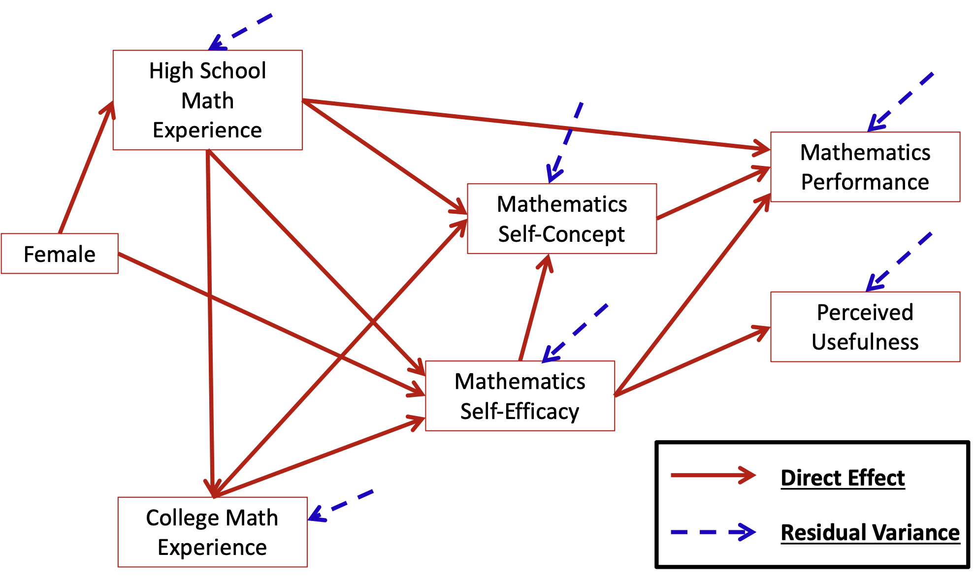
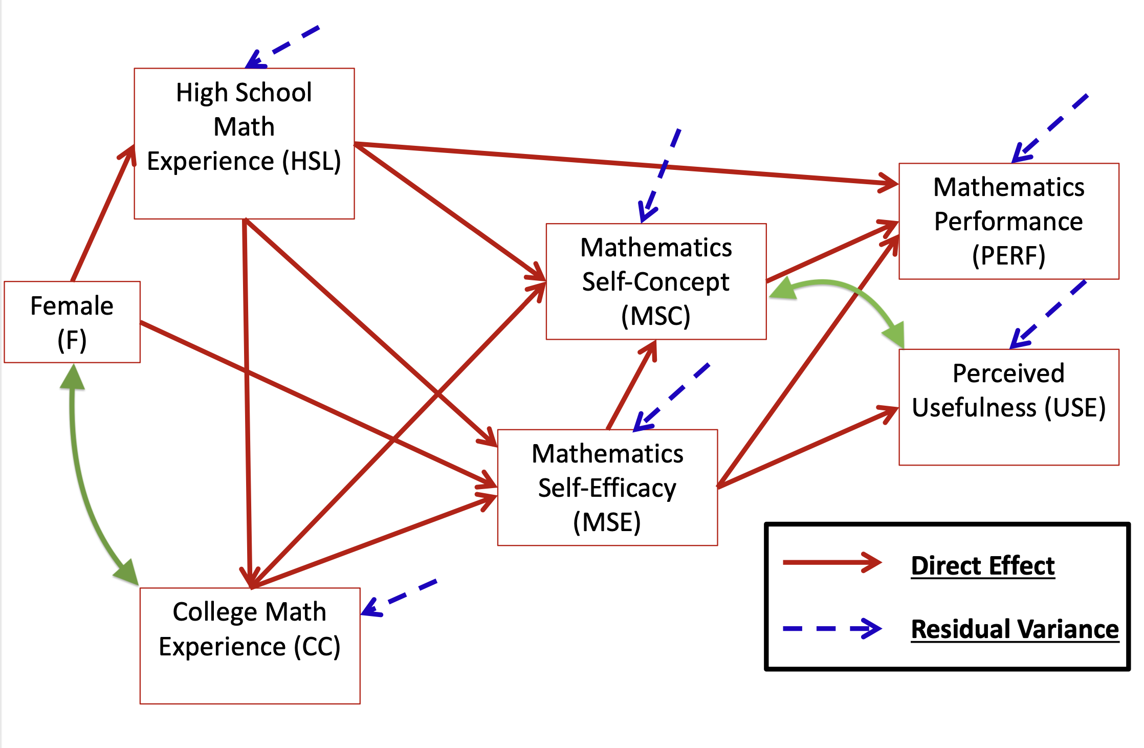
Multivariate Linear Regression Path Diagram

The Big Picture

Path analysis is a multivariate statistical method that, when using an identity link, assumes the variables in an analysis are multivariate normally distributed
- Mean vectors
- Covariance matrices
By specifying simultaneous regression equations (the core of path models), a very specific covariance matrix is implied
- This is where things deviate from our familiar R matrix
Like multivariate models, the key to path analysis is finding an approximation to the unstructured (saturated) covariance matrix
- With fewer parameters, if possible
The art to path analysis is in specifying models that blend theory and statistical evidence to produce valid, generalizable results

Types of Variables in Path Model

Endogenous variable(s): variables whose variability is explained by one or more variables in a model
- In linear regression, the dependent variable is the only endogenous variable in an analysis
  - Mathematics Performance (PERF) and Mathematics Usefulness (USE)
Exogenous variable(s): variables whose variability is not explained by any variables in a model
- In linear regression, the independent variable(s) are the exogenous variables in the analysis
  - Female (F)

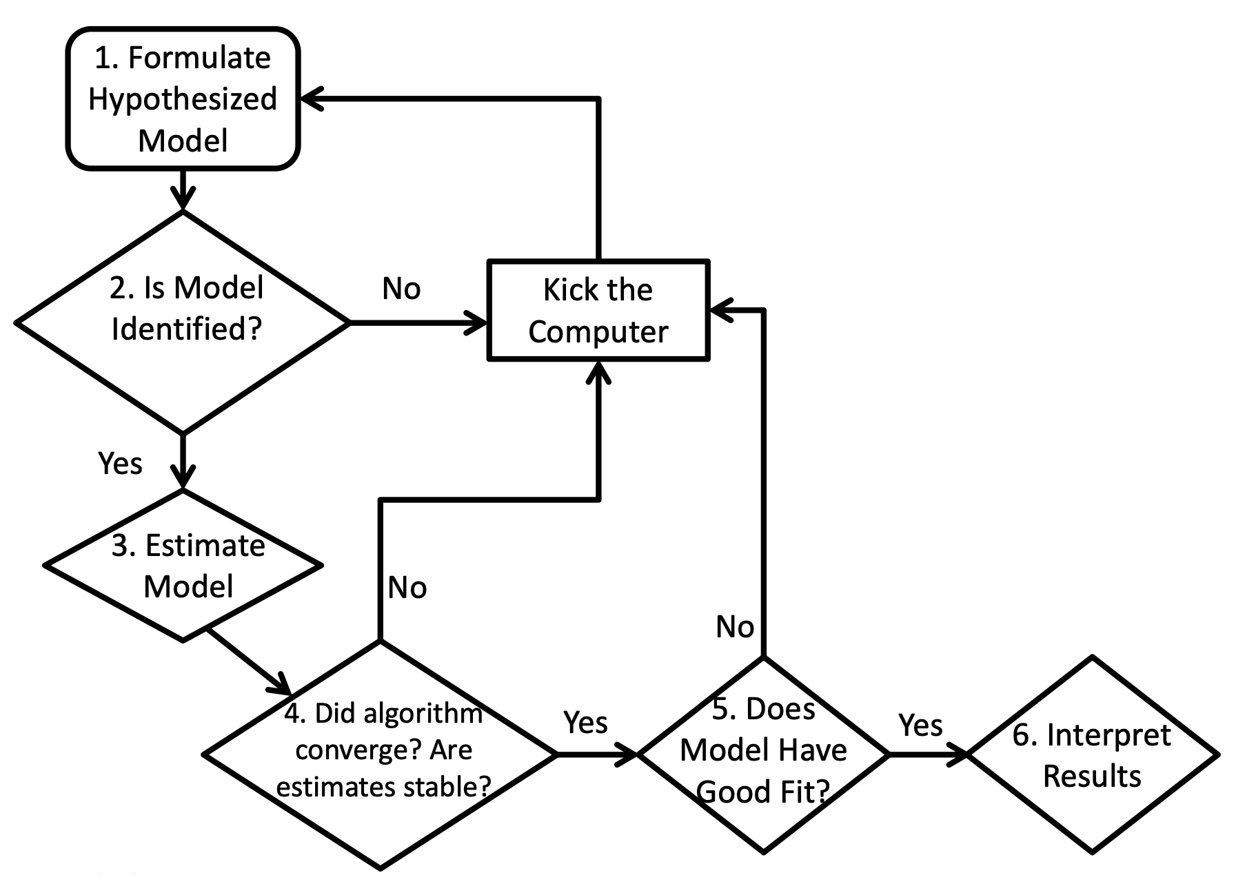
Procedure of Path Analysis Steps

Identification of Path Models

Model identification is necessary for statistical models to have “meaningful” results
For path models, identification can be very difficult
Because of their unique structure, path models must have identification in two ways:
- “Globally” – so that the total number of parameters does not exceed the total number of means, variances, and covariances of the endogenous and exogenous variables
- “Locally” – so that each individual equation is identified
Model identification is guaranteed if a model is both “globally” and “locally” identified

Global Identification: “T-rule”

A necessary but not sufficient condition for a path models is that of having equal to or fewer model parameters than there are “distributional parameters”
Distributional parameters: As the path models we discuss assume the multivariate normal distribution, we have two matrices of parameters
- The mean vector
- The covariance matrix
For the MVN, the so-called T-rule states that a model must have equal to or fewer parameters than the unique elements of the covariance matrix of all endogenous and exogenous variables (the sum of all variables in the analysis)
- Let s = p+q, the total of all endogenous (p) and exogenous (q) variables
- Then the total unique elements are $

T-rule Identification Status

Just-identified: number of observed covariances = number of model parameters
- Necessary for identification, but no model fit indices available
Over-identified: number of observed covariances > number of model parameters
- Necessary for identification; model fit indices available
Under-identified: number of observed covariances < number of model parameters
- Model is NOT IDENTIFIED: No results available

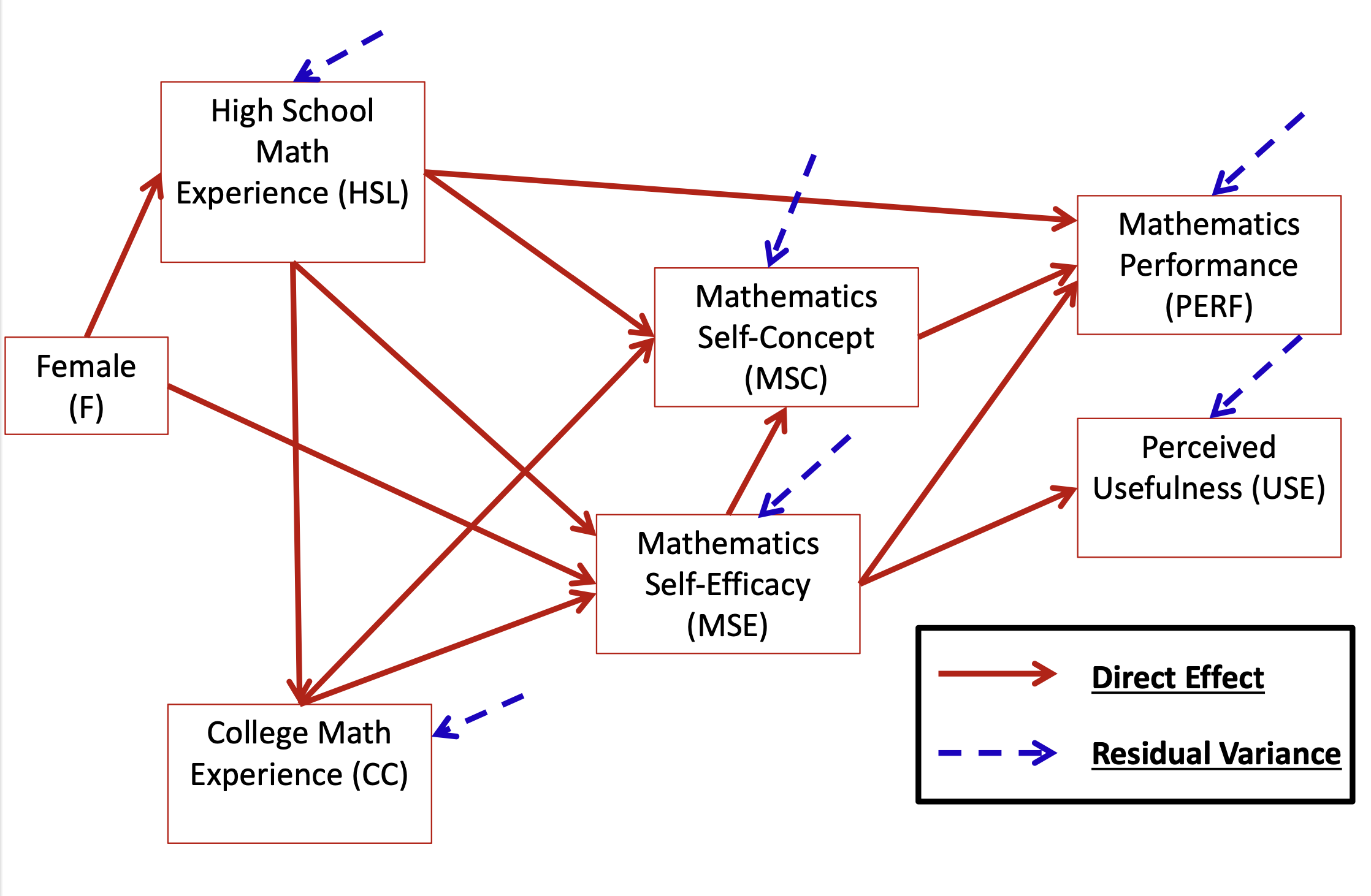
Our Destination: Overall Path Model

Based on the theory described in the introduction to Pajares & Miller (1994), the following model was hypothesized – use this diagram to build your knowledge of path models

Pajares, F., & Miller, M. D. (1994). Role of self-efficacy and self-concept beliefs in mathematical problem solving: A path analysis. Journal of Educational Psychology, 86(2), 193–203. https://doi.org/10.1037/0022-0663.86.2.193

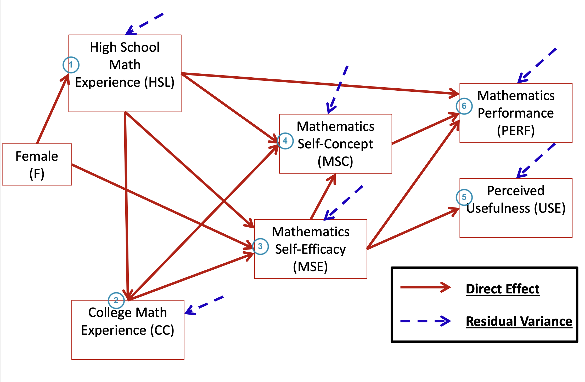
Overall Path Model: How to Inspect

Path Model Setup - Questions for the Analysis

How many variables are in our model? s = 7
- Gender, HSL, CC, MSC, MSE, PERF, and USE
How many variables are endogenous? p = 6
- HSL, CC, MSC, MSE, PERF and USE
How many variables are exogenous? q = 1
- Gender
Is the model recursive or non-recursive?
- Recursive – no feedback loops present

Path Model Setup – Questions for the Analysis

Is the model identified?
- Check the t-rule first
- How many covariance terms are there in the all-variable matrix?
  - \frac{7*(7+1)}{2} = 28
- How many model parameters are to be estimated?
  - 12 direct paths
  - 6 residual variances (only endogenous variables have resid. var.)
  - 1 variance of the exogenous variable
  - 6 endogenous variance intercepts
    - Not relevant for T-rule identification, but counted in R matrix
28 (total variances/covariances) > (12 + 6 + 1) parameters, thus this model is over-identified
- We can use R to run analysis

Overall Hypothesized Path Model: Equation Form

The path model from can be re-expressed in the following 6 endogenous variable regression equations:

HSL_i = \beta_{0, HSL} + \beta_{F, HSL}F_i + e_{i, HSL} \tag{1}

CC_i = \beta_{0,CC}+\beta_{HSL,CC}HSL_i + e_{i,CC} \tag{2}

MSE_i = \beta_{0,MSE} + \beta_{F,MSE}F_i +\beta_{HSL,MSE}HSL_i + \beta_{CC,MSE}CC_i +e_{i,MSE} \tag{3}

MSC_i = \beta_{0, MSE} + \beta_{HSL,MSC}HSL_i + \beta_{CC,MSC} CC_i + \beta_{MSE,MSC} MSE_i + e_{i,MSC} \tag{4}

USE_i = \beta_{0,USE} + \beta_{MSE,USE}MSE_{i} + e_{i, USE} \tag{5}

PERF_i = \beta_{0,PERF} + \beta_{HSL,PERF}HSL_{i} +\beta_{MSE,PERF}MSE_i + \beta_{MSC, PERF}MSC_{i} + e_{i,PERF} \tag{6}

Data Analytic Plan

Constructed our model
Verified it was identified using the t-rule and that it is a recursive model
Estimate the model with R
Check model fit

Path Model: `lavaan` syntax

#model 01-----------------------------------------------------------------------
model01.syntax = 
" 
#endogenous variable equations
perf ~ hsl + msc + mse
use  ~ mse
mse  ~ hsl + cc + female 
msc  ~ mse + cc + hsl
cc   ~ hsl
hsl  ~ female

#endogenous variable intercepts
perf ~ 1
use  ~ 1
mse  ~ 1
msc  ~ 1
cc   ~ 1
hsl  ~ 1

#endogenous variable residual variances
perf ~~ perf
use  ~~ use
mse  ~~ mse
msc  ~~ msc
cc   ~~ cc  
hsl  ~~ hsl

#endogenous variable residual covariances
#none specfied in the original model so these have zeros:
perf ~~ 0*use + 0*mse + 0*msc + 0*cc + 0*hsl
use  ~~ 0*mse + 0*msc + 0*cc + 0*hsl
mse  ~~ 0*msc + 0*cc + 0*hsl
msc  ~~ 0*cc + 0*hsl
cc   ~~ 0*hsl
"

Model Fit Evaluation

First, we check convergence:
- lavaan’s ML algorithm converged!

#estimate model
model01.fit = sem(model01.syntax, data=dataMath, mimic = "MPLUS", estimator = "MLR")

#see if model converged
inspect(model01.fit, what="converged")

[1] TRUE

Second, we check for abnormally large standard errors:

None too big, relative to the size of the parameter

Indicates identified mdoel

parameterestimates(model01.fit) |> filter(op != "~~")

      lhs op    rhs     est    se      z pvalue ci.lower ci.upper
1    perf  ~    hsl   0.172 0.107  1.600  0.110   -0.039    0.383
2    perf  ~    msc   0.036 0.009  3.981  0.000    0.018    0.054
3    perf  ~    mse   0.139 0.013 10.522  0.000    0.113    0.164
4     use  ~    mse   0.290 0.072  4.014  0.000    0.149    0.432
5     mse  ~    hsl   4.103 0.407 10.085  0.000    3.305    4.900
6     mse  ~     cc   0.393 0.105  3.729  0.000    0.186    0.599
7     mse  ~ female   4.285 1.159  3.697  0.000    2.013    6.557
8     msc  ~    mse   0.721 0.068 10.557  0.000    0.587    0.855
9     msc  ~     cc   0.557 0.132  4.211  0.000    0.298    0.817
10    msc  ~    hsl   2.929 0.659  4.446  0.000    1.638    4.220
11     cc  ~    hsl   0.681 0.246  2.771  0.006    0.199    1.163
12    hsl  ~ female   0.201 0.154  1.307  0.191   -0.101    0.504
13   perf ~1          1.009 0.788  1.281  0.200   -0.535    2.552
14    use ~1         31.118 5.357  5.809  0.000   20.619   41.618
15    mse ~1         47.885 2.246 21.319  0.000   43.482   52.287
16    msc ~1        -23.322 4.542 -5.135  0.000  -32.224  -14.419
17     cc ~1          6.979 1.263  5.524  0.000    4.503    9.455
18    hsl ~1          4.844 0.091 53.434  0.000    4.666    5.021
19 female ~1          0.346 0.000     NA     NA    0.346    0.346

Third, we look at the model fit statistics.

Model Fit Statistics

Before we interpret the estimation result, we need to assess the fit of a multivariate linear model to the data, in an absolute sense
If a model does not fit the data:
- Parameter estimates may be biased
- Standard errors of estimates may be biased
- Inferences made from the model may be wrong
- If the saturated model fit is wrong, then the LRTs will be inaccurate
Not all “good-fitting” models are useful…
- …model fit just allows you to talk about your model…there may be nothing of significance (statistically or practically) in your results, though

Global measures of Model fit

Root Mean Square Error of Approximation (RMSEA)
Likelihood ratio test
- User model versus the saturated model: Testing if your model fits as well as the saturated model
- The saturated model versue the baseline model: Testing whether any variables have non-zero covariances (significant correlations)
User model versus baseline model
- CFI (the comparative fit index)
- TLI (the Tucker–Lewis index)
Log-likelihood and Information Criteria
Standardized Root Mean Square Residual (SRMR)
- How far off a model’s correlations are from the saturated model correlations

Model Fit Statistics: Example

summary(model01.fit, fit.measures = TRUE)

1Model Test User Model:
                                              Standard      Scaled
  Test Statistic                                58.896      58.913
  Degrees of freedom                                 9           9
  P-value (Chi-square)                           0.000       0.000
  Scaling correction factor                                  1.000
    Yuan-Bentler correction (Mplus variant)                       

2Model Test Baseline Model:

  Test statistic                               619.926     629.882
  Degrees of freedom                                21          21
  P-value                                        0.000       0.000
  Scaling correction factor                                  0.984

3Root Mean Square Error of Approximation:

  RMSEA                                          0.126       0.126
  90 Percent confidence interval - lower         0.096       0.096
  90 Percent confidence interval - upper         0.157       0.157
  P-value H_0: RMSEA <= 0.050                    0.000       0.000
  P-value H_0: RMSEA >= 0.080                    0.994       0.994  
  
4User Model versus Baseline Model:

  Comparative Fit Index (CFI)                    0.917       0.918
  Tucker-Lewis Index (TLI)                       0.806       0.809
                                                                  
  Robust Comparative Fit Index (CFI)                         0.918
  Robust Tucker-Lewis Index (TLI)                            0.809

Loglikelihood and Information Criteria:

  Loglikelihood user model (H0)              -5889.496   -5889.496
  Scaling correction factor                                  0.965
      for the MLR correction                                      
  Loglikelihood unrestricted model (H1)      -5860.048   -5860.048
  Scaling correction factor                                  0.975
      for the MLR correction                                      
                                                                  
  Akaike (AIC)                               11826.992   11826.992
  Bayesian (BIC)                             11919.583   11919.583
  Sample-size adjusted Bayesian (SABIC)      11843.446   11843.446

1: This is a likelihood ratio (deviance) test comparing our model (H_0) with the saturated model – the saturated model fits much better (\chi^2(\Delta df = 9) = 58.896, p < .001)
2: This is a likelihood ratio (deviance) test comparing the baseline model with the saturated model
3: The RMSEA estimate is 0.126. Good fit is considered 0.05 or less.
4: The CFI estimate is .917 and the TLI is .806. Good fit is considered 0.95 or higher.

Based on the model fit statistics, we can conclude that our model does not do a good job of approximating the covariance matrix – so we cannot make inferences with these results (biased standard errors and effects may occur)

Model Modification Method 1: Check Residual Covariance

Now that we have concluded that our model fit is poor we must modify the model to make the fit better
- Our modifications are purely statistical – which draws into question their generalizability beyond this sample

Generally, model modification should be guided by theory

However, we can inspect the normalized residual covariance matrix (like z- scores) to see where our biggest misfit occurs
One normalized residual covariance is bigger than +/-1.96: MSC with USE and CC with Female

residuals(model01.fit, type = "normalized")

$type
[1] "normalized"

$cov
         perf    use    mse    msc     cc    hsl female
perf   -0.076                                          
use    -0.159  0.041                                   
mse    -0.071 -0.110 -0.086                            
msc     0.059  5.051 -0.039  0.043                     
cc     -0.028  0.720 -0.377 -0.161  0.046              
hsl     0.006  0.559  0.085  0.105 -0.034  0.039       
female -1.523 -0.027 -0.425 -1.452 -2.577  0.091  0.000

$mean
  perf    use    mse    msc     cc    hsl female 
-0.014  0.126  0.012  0.211  0.009  0.004  0.000

Our Destination: Overall Path Model

The largest normalized covariances suggest relationships that may be present that are not being modeled:
- Add a direct effect between F and CC
- Add a direct effect between MSC and USE OR Add a residual covariance between MSC and USE

Model Midification Method 2: More Help for Fit

As we used Maximum Likelihood to estimate our model, another useful feature is that of the modification indices
- Modification indices (also called Score or LaGrangian Multiplier tests) that attempt to suggest the change in the log-likelihood for adding a given model parameter (larger values indicate a better fit for adding the parameter)

#calculate modification indices
model01.mi = modificationindices(model01.fit, sort. = T)

#display values of indices
head(model01.mi, 10)

      lhs op    rhs     mi    epc sepc.lv sepc.all sepc.nox
54    msc  ~    use 41.517  0.299   0.299    0.275    0.275
31    use ~~    msc 41.517 70.912  70.912    0.386    0.386
46    use  ~    msc 40.032  0.451   0.451    0.490    0.490
63    hsl  ~    mse  6.486  1.139   1.139   10.265   10.265
65    hsl  ~     cc  6.477  0.447   0.447    1.992    1.992
39     cc ~~    hsl  6.477 15.131  15.131    1.974    1.974
59     cc  ~    msc  6.477 -0.568  -0.568   -1.654   -1.654
60     cc  ~ female  6.477 -1.756  -1.756   -0.142   -0.298
70 female  ~     cc  6.477 -0.012  -0.012   -0.145   -0.145
68 female  ~    mse  6.477 -0.030  -0.030   -0.748   -0.748

The modification indices have three large values:
- A direct effect predicting MSC from USE
- A direct effect predicting USE from MSC
- A residual covariance between USE and MSC
Note: the MI value is -2 times the change in the log-likelihood and the EPC is the expected parameter value
- The MI is like a 1 DF Chi-Square Deviance test
  - Values greater than 3.84 are likely to be significant changes in the log-likelihood
All three are for the same variable: so we can only choose one
- This is where theory would help us decide
As we do not know theory, we will choose to add a residual covariance between USE and MSC ( the “~~” symbol)
- Their covariance is unexplained by the model – not a great theoretical statement (but will allow us to make inferences if the model fits)
- MI = 41.517
- EPC = 70.912

Model 2: New Model by adding MSE with USE

Model 2: `lavaan` syntax

#model 02: Add residual covariance between USE and MSC-------------------------------------
model02.syntax = 
" 
#endogenous variable equations
perf ~ hsl + msc + mse
use  ~ mse
mse  ~ hsl + cc + female 
msc  ~ mse + cc + hsl
cc   ~ hsl
hsl  ~ female

#endogenous variable intercepts
perf ~ 1
use  ~ 1
mse  ~ 1
msc  ~ 1
cc   ~ 1
hsl  ~ 1

#endogenous variable residual variances
perf ~~ perf
use  ~~ use
mse  ~~ mse
msc  ~~ msc
cc   ~~ cc  
hsl  ~~ hsl

#endogenous variable residual covariances
#none specfied in the original model so these have zeros:
perf ~~ 0*use + 0*mse + 0*msc + 0*cc + 0*hsl
use  ~~ 0*mse + msc + 0*cc + 0*hsl      #<- the changed part of syntax here (no 0* in front of msc)
mse  ~~ 0*msc + 0*cc + 0*hsl
msc  ~~ 0*cc + 0*hsl
cc   ~~ 0*hsl
"

Assessing Model fit of the Modified Model

#estimate model
model02.fit = sem(model02.syntax, data=dataMath, mimic = "MPLUS", estimator = "MLR")

summary(model02.fit, standardized = TRUE)

lavaan 0.6-19 ended normally after 80 iterations

  Estimator                                         ML
  Optimization method                           NLMINB
  Number of model parameters                        25

  Number of observations                           350
  Number of missing patterns                        26

Model Test User Model:
                                              Standard      Scaled
  Test Statistic                                14.827      14.393
  Degrees of freedom                                 8           8
  P-value (Chi-square)                           0.063       0.072
  Scaling correction factor                                  1.030
    Yuan-Bentler correction (Mplus variant)                       

Parameter Estimates:

  Standard errors                             Sandwich
  Information bread                           Observed
  Observed information based on                Hessian

Regressions:
                   Estimate  Std.Err  z-value  P(>|z|)   Std.lv  Std.all
  perf ~                                                                
    hsl               0.153    0.107    1.432    0.152    0.153    0.068
    msc               0.037    0.009    4.147    0.000    0.037    0.215
    mse               0.139    0.013   10.700    0.000    0.139    0.557
  use ~                                                                 
    mse               0.277    0.073    3.803    0.000    0.277    0.209
  mse ~                                                                 
    hsl               4.138    0.406   10.203    0.000    4.138    0.459
    cc                0.393    0.105    3.723    0.000    0.393    0.194
    female            4.168    1.160    3.593    0.000    4.168    0.166
  msc ~                                                                 
    mse               0.736    0.066   11.119    0.000    0.736    0.512
    cc                0.519    0.117    4.434    0.000    0.519    0.179
    hsl               2.824    0.593    4.764    0.000    2.824    0.218
  cc ~                                                                  
    hsl               0.662    0.247    2.686    0.007    0.662    0.149
  hsl ~                                                                 
    female            0.208    0.154    1.348    0.178    0.208    0.075

Covariances:
                   Estimate  Std.Err  z-value  P(>|z|)   Std.lv  Std.all
 .perf ~~                                                               
   .use               0.000                               0.000    0.000
   .mse               0.000                               0.000    0.000
   .msc               0.000                               0.000    0.000
   .cc                0.000                               0.000    0.000
   .hsl               0.000                               0.000    0.000
 .use ~~                                                                
   .mse               0.000                               0.000    0.000
   .msc              70.249   10.358    6.782    0.000   70.249    0.380
   .cc                0.000                               0.000    0.000
   .hsl               0.000                               0.000    0.000
 .mse ~~                                                                
   .msc               0.000                               0.000    0.000
   .cc                0.000                               0.000    0.000
   .hsl               0.000                               0.000    0.000
 .msc ~~                                                                
   .cc                0.000                               0.000    0.000
   .hsl               0.000                               0.000    0.000
 .cc ~~                                                                 
   .hsl               0.000                               0.000    0.000

Intercepts:
                   Estimate  Std.Err  z-value  P(>|z|)   Std.lv  Std.all
   .perf              1.023    0.782    1.309    0.191    1.023    0.344
   .use              32.162    5.393    5.964    0.000   32.162    2.035
   .mse              47.738    2.237   21.339    0.000   47.738    4.006
   .msc             -23.369    4.484   -5.211    0.000  -23.369   -1.364
   .cc                7.072    1.268    5.576    0.000    7.072    1.201
   .hsl               4.843    0.091   53.390    0.000    4.843    3.663

Variances:
                   Estimate  Std.Err  z-value  P(>|z|)   Std.lv  Std.all
   .perf              3.763    0.309   12.173    0.000    3.763    0.427
   .use             238.854   19.097   12.507    0.000  238.854    0.956
   .mse              97.294    7.758   12.541    0.000   97.294    0.685
   .msc             142.912   10.793   13.241    0.000  142.912    0.487
   .cc               33.923    2.456   13.813    0.000   33.923    0.978
   .hsl               1.738    0.126   13.813    0.000    1.738    0.994

#see if model converged
inspect(model02.fit, what="converged")

[1] TRUE

#show summary of model fit statistics and parameters
summary(model02.fit, standardized=TRUE, fit.measures=TRUE)

needed_fitIndex <- c("rmsea", "srmr","cfi", "tli", "chisq", "df", "pvalue") 
fitmeasures(model02.fit)[needed_fitIndex]

      rmsea        srmr         cfi         tli       chisq          df 
 0.04937683  0.03459811  0.98860192  0.97008004 14.82660076  8.00000000 
     pvalue 
 0.06260610

Now we must start over with our path model decision tree
- The model is identified (now 20 parameters < 28 covariances)
- Estimation converged; Standard errors look acceptable
Model fit indices:
- The comparison with the saturated model suggests our model fits statistically
- The RMSEA is 0.049, which indicates good fit
- The CFI and TLI both indicate good fit (CFI/TLI > .90)
- The SRMR also indicates good fit
Therefore, we can conclude the model adequately approximates the covariance matrix – meaning we can now inspect our model parameters…but first, let’s check our residual covariances and modification indices

Normalized Residual Covariances

residuals(model02.fit, type = "normalized")

$type
[1] "normalized"

$cov
         perf    use    mse    msc     cc    hsl female
perf   -0.062                                          
use    -0.990  0.020                                   
mse    -0.113  0.064 -0.103                            
msc    -0.003  0.337 -0.104  0.054                     
cc      0.018  0.771 -0.355  0.050  0.034              
hsl     0.062  0.638  0.020  0.154  0.037  0.017       
female -1.500  0.026 -0.362 -1.456 -2.577  0.051  0.000

$mean
  perf    use    mse    msc     cc    hsl female 
-0.013  0.066  0.028  0.044  0.003 -0.015  0.000

Only one normalized residual covariance is bigger than +/- 1.96: CC with Female
- Given the number of covariances we have, this is likely okay

Modeification Indices for Model 2

model02.mi = modificationindices(model02.fit, sort. = T)
head(model02.mi, 10)

      lhs op    rhs    mi    epc sepc.lv sepc.all sepc.nox
39     cc ~~    hsl 6.697 14.964  14.964    1.949    1.949
68 female  ~    mse 6.697 -0.030  -0.030   -0.761   -0.761
70 female  ~     cc 6.697 -0.012  -0.012   -0.148   -0.148
60     cc  ~ female 6.697 -1.788  -1.788   -0.144   -0.304
58     cc  ~    mse 6.697 -0.429  -0.429   -0.868   -0.868
65    hsl  ~     cc 6.697  0.441   0.441    1.965    1.965
63    hsl  ~    mse 6.696  1.124   1.124   10.128   10.128
66 female  ~   perf 5.126 -0.032  -0.032   -0.199   -0.199
61    hsl  ~   perf 4.410  0.774   0.774    1.739    1.739
69 female  ~    msc 4.405 -0.004  -0.004   -0.162   -0.162

Now, no modification indices are glaringly large, although some are bigger than 3.84
- We discard these as our model now fits (and adding them may not be meaningful)

More on Modification Indices

Recall from our original model that we received the following modification index values for the residual covariance between MSC and USE:
- MI = 41.529
- EPC = 70.912

model01.mi[2, ]

   lhs op rhs     mi    epc sepc.lv sepc.all sepc.nox
31 use ~~ msc 41.517 70.912  70.912    0.386    0.386

The estimated residual covariance between MSC and USE in the modified model is: 70.249

parameterestimates(model02.fit) |> filter(lhs == "use"& op == "~~"& rhs == "msc")

  lhs op rhs    est     se     z pvalue ci.lower ci.upper
1 use ~~ msc 70.249 10.358 6.782      0   49.947   90.551

The difference in log-likelihoods is:
- -2*(change) = 58.279

anova(model01.fit, model02.fit)


Scaled Chi-Squared Difference Test (method = "satorra.bentler.2001")

lavaan->lavTestLRT():  
   lavaan NOTE: The "Chisq" column contains standard test statistics, not the 
   robust test that should be reported per model. A robust difference test is 
   a function of two standard (not robust) statistics.
            Df   AIC   BIC  Chisq Chisq diff Df diff Pr(>Chisq)    
model02.fit  8 11785 11881 14.827                                  
model01.fit  9 11827 11920 58.896     58.279       1  2.275e-14 ***
---
Signif. codes:  0 '***' 0.001 '**' 0.01 '*' 0.05 '.' 0.1 ' ' 1

The values given by the MI and EPC are approximations

Model Parameter Investigation

Regressions:
                   Estimate  Std.Err  z-value  P(>|z|)   Std.lv  Std.all
  perf ~                                                                
    hsl               0.153    0.107    1.432    0.152    0.153    0.068
    msc               0.037    0.009    4.147    0.000    0.037    0.215
    mse               0.139    0.013   10.700    0.000    0.139    0.557
  use ~                                                                 
    mse               0.277    0.073    3.803    0.000    0.277    0.209
  mse ~                                                                 
    hsl               4.138    0.406   10.203    0.000    4.138    0.459
    cc                0.393    0.105    3.723    0.000    0.393    0.194
    female            4.168    1.160    3.593    0.000    4.168    0.166
  msc ~                                                                 
    mse               0.736    0.066   11.119    0.000    0.736    0.512
    cc                0.519    0.117    4.434    0.000    0.519    0.179
    hsl               2.824    0.593    4.764    0.000    2.824    0.218
  cc ~                                                                  
    hsl               0.662    0.247    2.686    0.007    0.662    0.149
  hsl ~                                                                 
    female            0.208    0.154    1.348    0.178    0.208    0.075

There are two direct effects that are non-significant:
- \beta_{F, HSL} = .208, p = .178
- \beta_{HSL, PERF} = .153, p = .152
We leave these in the model 2, but the overall path model seems to suggest they are not needed
- So, I will remove them and re-estimate the model

Model 3: Remove non-significant effects

Model 3: `lavaan` syntax

#model 03: removing HSL predicting PERF and Gender predicting HSL  ----------------
model03.syntax = 
" 
#endogenous variable equations
perf ~ msc + mse
use  ~ mse
mse  ~ hsl + cc + female 
msc  ~ mse + cc + hsl
cc   ~ hsl

#endogenous variable intercepts
perf ~ 1
use  ~ 1
mse  ~ 1
msc  ~ 1
cc   ~ 1

#endogenous variable residual variances
perf ~~ perf
use  ~~ use
mse  ~~ mse
msc  ~~ msc
cc   ~~ cc  

#endogenous variable residual covariances
#none specfied in the original model so these have zeros:
perf ~~ 0*use + 0*mse + 0*msc + 0*cc 
use  ~~ 0*mse + msc + 0*cc  
mse  ~~ 0*msc + 0*cc 
msc  ~~ 0*cc 
"

#estimate model
model03.fit = sem(model03.syntax, data=dataMath, mimic = "MPLUS", estimator = "MLR")
summary(model03.fit, fit.measures = TRUE)

Model 3: Model fit results

We have: an identified model, a converged algorithm, and stable standard errors, so model fit should be inspected
- Next – inspect model fit
- Model fit seems to not be as good as we would think

#see if model converged
inspect(model03.fit, what="converged")

[1] TRUE

fitmeasures(model03.fit)[needed_fitIndex]

      rmsea        srmr         cfi         tli       chisq          df 
 0.05739989  0.03674047  0.98265706  0.96146014 18.31095521  9.00000000 
     pvalue 
 0.03173258

Again, the largest normalized residual covariance is that of Female and CC

residuals(model03.fit, type = "normalized")

$type
[1] "normalized"

$cov
         perf    use    mse    msc     cc    hsl female
perf   -0.063                                          
use    -1.380  0.025                                   
mse    -0.140  0.129 -0.113                            
msc     0.024  0.303 -0.084  0.065                     
cc     -0.394  0.417 -0.282  0.006  0.017              
hsl     0.949  0.626 -0.055  0.138  0.010  0.000       
female -1.531  0.332 -0.329 -1.886 -2.241  0.000  0.000

$mean
  perf    use    mse    msc     cc    hsl female 
-0.033  0.073  0.024  0.068 -0.014  0.000  0.000

MI for direct effect of Female on CC is 5.090, indicating that adding this parameter may improve model fit

modificationindices(model03.fit, sort. = T)[1:3,]

    lhs op    rhs    mi    epc sepc.lv sepc.all sepc.nox
36 perf  ~    use 5.625 -0.021  -0.021   -0.111   -0.111
21 perf ~~    use 5.238 -4.264  -4.264   -0.139   -0.139
55   cc  ~ female 5.090 -1.653  -1.653   -0.133   -0.278

So, we will now add a direct effect of Female on CC

Model 4: Adding Female on CC

Model 4: `lavaan` syntax

#model 04: Add gender predicting cc -------------------------------------------------------------
model04.syntax = " 
#endogenous variable equations
perf ~ msc + mse
use  ~ mse
mse  ~ (b_hsl_mse)*hsl + (b_cc_mse)*cc + female 
msc  ~ mse + cc + hsl
cc   ~ (b_hsl_cc)*hsl + female

#endogenous variable intercepts
perf ~ 1
use  ~ 1
mse  ~ 1
msc  ~ 1
cc   ~ 1

#endogenous variable residual variances
perf ~~ perf
use  ~~ use
mse  ~~ mse
msc  ~~ msc
cc   ~~ cc  

#endogenous variable residual covariances
#none specfied in the original model so these have zeros:
perf ~~ 0*use + 0*mse + 0*msc + 0*cc 
use  ~~ 0*mse + msc + 0*cc  
mse  ~~ 0*msc + 0*cc 
msc  ~~ 0*cc 

#indirect effect of interest:
ind_hsl_mse := b_hsl_cc*b_cc_mse

#total effect of interest:
tot_hsl_mse := b_hsl_mse + (b_hsl_cc*b_cc_mse)
"
model04.fit = sem(model04.syntax, data=dataMath, mimic = "MPLUS", estimator = "MLR")

Model 4: Model Fit Index

inspect(model04.fit, what="converged")

[1] TRUE

fitmeasures(model04.fit)[needed_fitIndex]

      rmsea        srmr         cfi         tli       chisq          df 
 0.04531236  0.02405819  0.99039314  0.97598285 13.15766273  8.00000000 
     pvalue 
 0.10653884

residuals(model04.fit, type = "normalized")

$type
[1] "normalized"

$cov
         perf    use    mse    msc     cc    hsl female
perf   -0.008                                          
use    -1.364  0.027                                   
mse    -0.055  0.150 -0.021                            
msc     0.100  0.320  0.019  0.125                     
cc     -0.193  0.476  0.017  0.093 -0.028              
hsl     0.951  0.625 -0.054  0.140  0.025  0.000       
female -1.107  0.417  0.125 -1.188  0.067  0.000  0.000

$mean
  perf    use    mse    msc     cc    hsl female 
-0.034  0.072  0.022  0.066  0.006  0.000  0.000

model04.mi <- modificationindices(model04.fit, sort. = T)
head(model04.mi, 5)

    lhs op    rhs    mi    epc sepc.lv sepc.all sepc.nox
39 perf  ~    use 5.624 -0.021  -0.021   -0.111   -0.111
22 perf ~~    use 5.237 -4.262  -4.262   -0.139   -0.139
43  use  ~   perf 4.860 -1.074  -1.074   -0.201   -0.201
53  msc  ~ female 3.243 -2.626  -2.626   -0.075   -0.156
58  hsl  ~   perf 2.449  0.078   0.078    0.178    0.178

We have: an identified model, a converged algorithm, and stable standard errors, so model fit should be inspected
No normalized residual covariances are larger than +/- 1.96 – so we appear to have good fit
We will leave this model as-is and interpret the results

Model 4: Parameter Interpretation

Interpret each of these parameters as you would in regression:
- A one-unit increase in HSL brings about a .695 unit increase in CC, holding Female constant
- We can interpret the standardized parameter estimates for all variables except gender
- A 1-SD increase in HSL means CC increases by 0.153 SD

parameterestimates(model04.fit, standardized = T, ci = F) |> filter(op == "~")

    lhs op    rhs     label    est    se      z pvalue std.lv std.all std.nox
1  perf  ~    msc            0.042 0.009  4.598  0.000  0.042   0.236   0.236
2  perf  ~    mse            0.151 0.013 11.353  0.000  0.151   0.586   0.586
3   use  ~    mse            0.279 0.079  3.513  0.000  0.279   0.203   0.203
4   mse  ~    hsl b_hsl_mse  4.050 0.410  9.869  0.000  4.050   0.456   0.347
5   mse  ~     cc  b_cc_mse  0.383 0.106  3.613  0.000  0.383   0.196   0.196
6   mse  ~ female            3.819 1.201  3.180  0.001  3.819   0.156   0.327
7   msc  ~    mse            0.692 0.070  9.872  0.000  0.692   0.481   0.481
8   msc  ~     cc            0.545 0.120  4.534  0.000  0.545   0.193   0.193
9   msc  ~    hsl            2.894 0.608  4.760  0.000  2.894   0.227   0.172
10   cc  ~    hsl  b_hsl_cc  0.695 0.254  2.737  0.006  0.695   0.153   0.117
11   cc  ~ female           -1.662 0.719 -2.312  0.021 -1.662  -0.133  -0.279

Model Interpretation: Explained Variability

sort(inspect(model04.fit, what = 'r2'))

        cc        use        mse        msc       perf 
0.03875216 0.04124687 0.29765620 0.48535191 0.57624994

The R2 for each endogenous variable:
- CC – 0.039
- USE – 0.041
- MSE – 0.298
- MSC – 0.485
- PERF – 0.576
Note how college experience and perceived usefulness both have low percentages of variance accounted for by the model
- We could have increased the R2 for USE by adding the direct path between MSC and USE instead of the residual covariance

Overall Model Interpretation

High School Experience and Female are significant predictors of College Experience (\beta_{HSL, CC} = .695, p = .006 and \beta_{F, CC} = -1.662, p = .021)
- Females lower than males in College Experience
- More High School Experience means more College Experience
High School Experience, College Experience, and Gender are significant predictors of Math Self-Efficacy (\beta_{HSL, MSE}= 4.05, p < .001; \beta_{CC, MSE}= .383, p < .001; \beta_{F, MSE}= 3.819, p = .001)
- More High School and College Experience means higher Math Self-Efficacy
- Females have higher Math Self-Efficacy than Men
High School Experience, College Experience, and Math Self-Efficacy are significant predictors of Math Self-Concept (\beta_{HSL, MSC}= 2.894, p < .001; \beta_{CC, MSC}= .545, p < .001; \beta_{MSE, MSC}= .692, p < .001)
- More High School and College Experience and higher Math Self-Efficacy mean higher Math Self-Concept
Higher Math Self-Efficacy means significantly higher Perceived Usefulness
Higher Math Self-Efficacy and Math Self-Concept result in higher Math Performance scores
Math Self-Concept and Perceived Usefulness have a significant residual covariance

Wrapping Up

In this lecture we discussed the basics of path analysis
- Model specification/identification
- Model estimation
- Model fit (necessary, but not sufficient)
- Model modification and re-estimation
- Final model parameter interpretation
There is a lot to the analysis – but what is important to remember is the over-arching principal of multivariate analyses: covariance between variables is important
- Path models imply very specific covariance structures
- The validity of the results hinge upon accurately finding an approximation to the covariance matrix

Next Class

Indirect effect
Causality
Hypothesis tests
Robust ML

Today’s Class

Today's Class

Path Analysis

Today’s Example Data

Multivariate Linear Regression Path Diagram

The Big Picture

Types of Variables in Path Model

Procedure of Path Analysis Steps

Identification of Path Models

Global Identification: “T-rule”

More on the “T-rule”

T-rule Identification Status

Our Destination: Overall Path Model

Overall Path Model: How to Inspect

Path Model Setup - Questions for the Analysis

Path Model Setup – Questions for the Analysis

Overall Hypothesized Path Model: Equation Form

Data Analytic Plan

Path Model: lavaan syntax

Model Fit Evaluation

Model Fit Statistics

Global measures of Model fit

Model Fit Statistics: Example

Model Modification Method 1: Check Residual Covariance

Our Destination: Overall Path Model

Model Midification Method 2: More Help for Fit

Model 2: New Model by adding MSE with USE

Model 2: lavaan syntax

Assessing Model fit of the Modified Model

Normalized Residual Covariances

Modeification Indices for Model 2

More on Modification Indices

Model Parameter Investigation

Model 3: Remove non-significant effects

Model 3: lavaan syntax

Model 3: Model fit results

Model 4: Adding Female on CC

Model 4: lavaan syntax

Model 4: Model Fit Index

Model 4: Parameter Interpretation

Model Interpretation: Explained Variability

Overall Model Interpretation

Wrapping Up

Next Class

Path Model: `lavaan` syntax

Model 2: `lavaan` syntax

Model 3: `lavaan` syntax

Model 4: `lavaan` syntax