---
title: 'Network analysis estimation for application research'
subtitle: 'Compare multiple R packages for psychological network analysis'
date: 'April 4 2024'
image: "index_files/figure-html/fig-bfi-1.png"
categories:
- R
- Bayesian
- Tutorial
- Network Analysis
execute:
eval: true
echo: true
warning: false
fig-align: center
format:
html:
code-fold: true
code-summary: 'Click to see the code'
toc-location: right
toc-depth: 2
toc-expand: true
bibliography: references.bib
csl: apa.csl
---
# Background
Multiple estimation methods for network analysis have been proposed, from regularized to unregularized, from frequentist to Bayesian approach, from one-step to multiple steps.
@isvoranuWhichEstimationMethod2023a provides an throughout illustration of current network estimation methods and simulation study.
This post tries to reproduce the procedures and coding illustrated by the paper and compare the results for packages with up-to-date version.
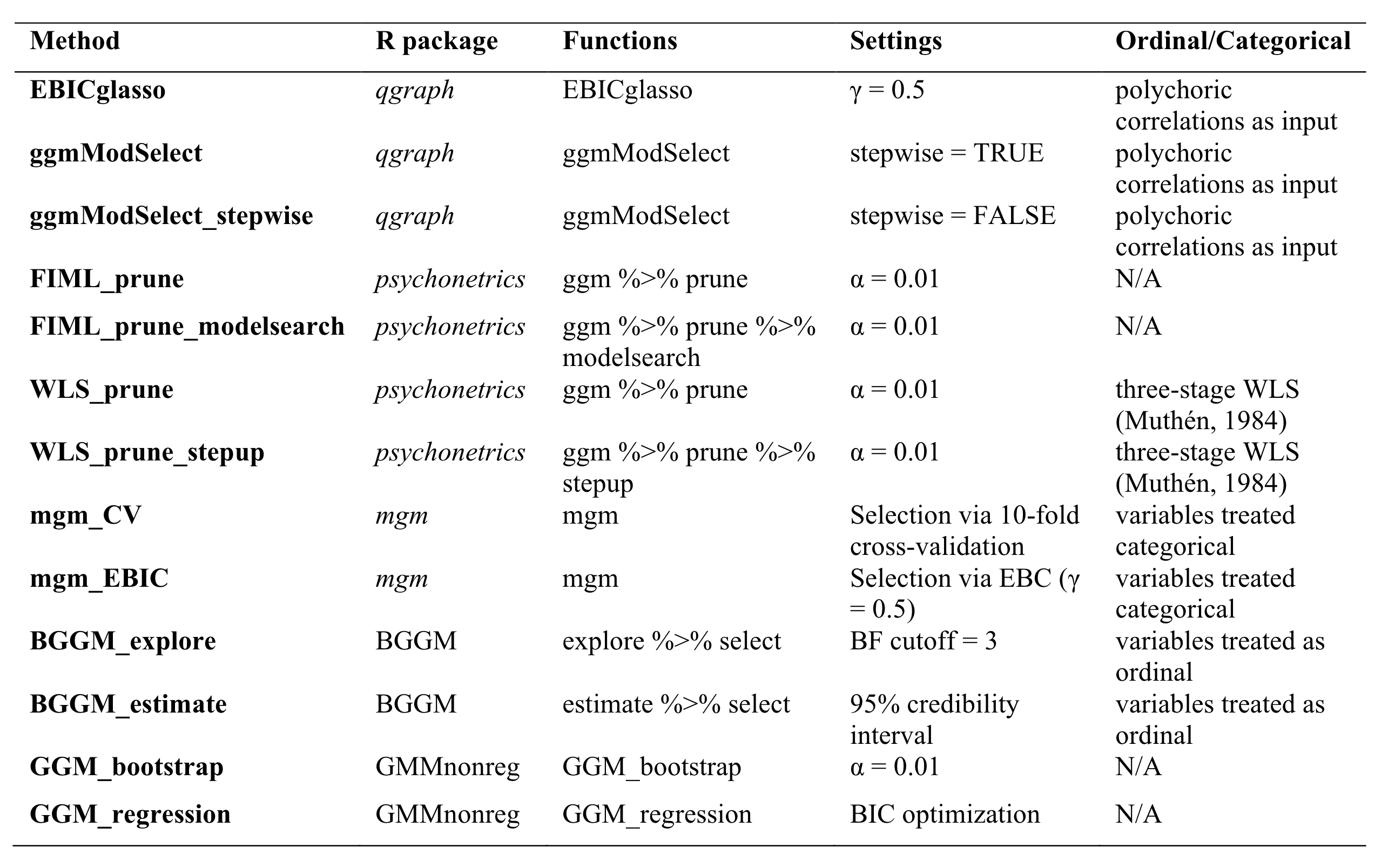
Five packages will be used for network modeling: (1) `qgraph`, (2)`psychonetrics`, (3)`MGM`, (4)`BGGM`, (5)`GGMnonreg`.
Note that the tutorial of each R package is not the scope of this post.
The specific variants of estimation is described in @fig-usedestimation.
Please see [here](../2024-03-05-Bayesian-GGM/index.qmd) for `BGGM` R package for more detailed example.
{#fig-usedestimation fig-align="center"}
# Simulation Study 1
## Data Generation
For the sake of simplicity, I will only pick one condition from the simulation settings.
To simulate data, I used the same code from the paper.
The function is a wrapper of `bootnet::ggmGenerator` function
```{r}
#| code-summary: 'dataGenerator() function'
library("bootnet")
library("qgraph")

mycolors = c("#4682B4", "#B4464B", "#752021",
             "#1B9E77", "#66A61E", "#D95F02", "#7570B3",
             "#E7298A", "#E75981", "#B4AF46", "#B4726A")

dataGenerator <- function(
  trueNet,  # true network models: DASS21, PTSD, BFI
  sampleSize, # sample size
  data = c("normal","skewed","uniform ordered","skewed ordered"), # type of data
  nLevels = 4,
  missing = 0
){
  data <- match.arg(data)
  nNode <- ncol(trueNet)

  if (data == "normal" || data == "skewed"){
    # Generator function:
    gen <- ggmGenerator()

    # Generate data:
    Data <- gen(sampleSize,trueNet)

    # Generate replication data:
    Data2 <- gen(sampleSize,trueNet)

    if (data == "skewed"){ ## exponential transformation to make data skewed
      for (i in 1:ncol(trueNet)){
        Data[,i] <- exp(Data[,i])
        Data2[,i] <- exp(Data2[,i])
      }
    }

  } else {
    # Skew factor:
    skewFactor <- switch(data,
                         "uniform ordered" = 1,
                         "skewed ordered" = 2,
                         "very skewed ordered" = 4)

    # Generator function:
    gen <- ggmGenerator(ordinal = TRUE, nLevels = nLevels)

    # Make thresholds:
    thresholds <- lapply(seq_len(nNode),function(x)qnorm(seq(0,1,length=nLevels + 1)[-c(1,nLevels+1)]^(1/skewFactor)))

    # Generate data:
    Data <- gen(sampleSize, list(
      graph = trueNet,
      thresholds = thresholds
    ))

    # Generate replication data:
    Data2 <- gen(sampleSize, list(
      graph = trueNet,
      thresholds = thresholds
    ))
  }

  # Add missings:
  if (missing > 0){
    for (i in 1:ncol(Data)){
      Data[runif(sampleSize) < missing,i] <- NA
      Data2[runif(sampleSize) < missing,i] <- NA
    }
  }

  return(list(
    data1 = Data,
    data2 = Data2
  ))
}
```
BFI contains 26 columns: first columns are the precision matrix with 25 $\times$ 25 and second columns as clusters.
We will use the structure of BFI for the simulation.
```{r}
library(here)
bfi_truenetwork <- read.csv(here("posts", "2024", "2024-04-04-Network-Estimation-Methods",
                                 "weights matrices", "BFI.csv"))
bfi_truenetwork <- bfi_truenetwork[,1:25]
head(psychTools::bfi)
```
To generate data from `bootnet::ggmGenerator()`, we can generate a function `gen` from it with first argument as sample size and second argument as partial correlation matrix.
```{r}
#| code-fold: show
gen <- bootnet::ggmGenerator()
data <- gen(2800, as.matrix(bfi_truenetwork))
```
## Measures
### Overview of Centrality Measures
Centrality measures are used as one characteristic of network model to summarize the importance of nodes/items given a network.
Some ideas of centrality measures come from social network.
Some may not make much sense in psychometric network.
I also listed the centrality measures that have been used in literatures of psychological or psychometric modeling.
Following the terminology of @christensen2018, centrality measures include: (1) betweenness centrality (BC); (2) the randomized shortest paths betweeness centrality (RSPBC); (3) closeness centrality (CC); (4)node degree (ND); (5) node strength (NS); (6) expected influence (EI); (7) engenvector centrality (EC); (8) Eccentricity (*k;* @hage1995); (9) hybrid centrality (HC; @christensen2018a).
They can be grouped into three categories:
[*Type 1*]{.underline}—Number of path relevant metrics: BC measures how often a node is on the shortest path from one node to another.
RSPBC is a adjusted BC measure which measures how oftern a node is on the random shortest path from one to another; CC measures the average number of paths from one node to all other nodes in the network.
ND measures how many connections are connected to each node.
Eccentricity (*k*) measures the maximum "distance" between one node with other nodes with lower values suggests higher centrality, where one node's distance is the length of a shortest path between this node to other nodes.
[*Type 2*]{.underline}—Path strength relevant metrics: **NS** measures the sum of the absolute values of edge weights connected to a single node.
**EI** measures the sum of the positive or negative values of edge weights connected to a single node.
[*Type 3*]{.underline}—Composite of multiple centrality measures: **HC** measures nodes on the basis of their centrality values across multiple measures of centrality (BC, LC, *k*, EC, and NS) which describes highly central nodes with large values and highly peripheral nodes with small values [@christensen2018b].
Some literature of network psychometrics criticized the use of Type 1 centrality measures and some Type II centrality measures [@hallquist2021; @neal2022].
For example, @hallquist2021 argued that some Type I centrality measures such as BC and CC derive from the concept of distance, which builds on the physical nature of many traditional graph theory applications, including railways and compute networks.
In association networks, the idea of network distance does not have physical reference.
@bringmann2019 also think distance-based centrality like closeness centrality (CC) and betweenness centrality (BC) do not have "shortest path", or "node exchangeability" assumptions in psychological networks so they are not suitable in the context of psychological network.
In addition, ND (degree), CC (closeness), and BC (betweenness) do not take negative values of edge weights into account that may lose important information in the context of psychology.
### Network level accuracy metrics
Structure accuracy measures such as *sensitivity*, specificity, and precision investigate if an true edge is include or not or an false edge is include or not.
Several edge weight accuracy measures include: (1) correlation between absolute values of estimated edge weights and true edge weights, (2) average absolute bias between estimated edge weights and true weights, (3) average absolute bias for true edges.
```{r}
cor0 <- function(x,y,...){
  if (sum(!is.na(x)) < 2 || sum(!is.na(y)) < 2 || sd(x,na.rm=TRUE)==0 | sd(y,na.rm=TRUE) == 0){
    return(0)
  } else {
    return(cor(x,y,...))
  }
}

bias <- function(x,y) mean(abs(x-y),na.rm=TRUE)


### Inner function:
comparison_metrics <- function(real, est, name = "full"){

  # Output list:
  out <- list()

  # True positives:
  TruePos <- sum(est != 0 &  real != 0)

  # False pos:
  FalsePos <- sum(est != 0 & real == 0)

  # True Neg:
  TrueNeg <- sum(est == 0 & real == 0)

  # False Neg:
  FalseNeg <- sum(est == 0 & real != 0)

  # Sensitivity:
  out$sensitivity <- TruePos / (TruePos + FalseNeg)

  # Sensitivity top 50%:
  top50 <- which(abs(real) > median(abs(real[real!=0])))
  out[["sensitivity_top50"]] <- sum(est[top50]!=0 & real[top50] != 0) / sum(real[top50] != 0)

  # Sensitivity top 25%:
  top25 <- which(abs(real) > quantile(abs(real[real!=0]), 0.75))
  out[["sensitivity_top25"]] <- sum(est[top25]!=0 & real[top25] != 0) / sum(real[top25] != 0)

  # Sensitivity top 10%:
  top10 <- which(abs(real) > quantile(abs(real[real!=0]), 0.90))
  out[["sensitivity_top10"]] <- sum(est[top10]!=0 & real[top10] != 0) / sum(real[top10] != 0)

  # Specificity:
  out$specificity <- TrueNeg / (TrueNeg + FalsePos)

  # Precision (1 - FDR):
  out$precision <- TruePos / (FalsePos + TruePos)

  # precision top 50% (of estimated edges):
  top50 <- which(abs(est) > median(abs(est[est!=0])))
  out[["precision_top50"]] <- sum(est[top50]!=0 & real[top50] != 0) / sum(est[top50] != 0)

  # precision top 25%:
  top25 <- which(abs(est) > quantile(abs(est[est!=0]), 0.75))
  out[["precision_top25"]] <- sum(est[top25]!=0 & real[top25] != 0) / sum(est[top25] != 0)

  # precision top 10%:
  top10 <- which(abs(est) > quantile(abs(est[est!=0]), 0.90))
  out[["precision_top10"]] <- sum(est[top10]!=0 & real[top10] != 0) / sum(est[top10] != 0)

  # Signed sensitivity:
  TruePos_signed <- sum(est != 0 &  real != 0 & sign(est) == sign(real))
  out$sensitivity_signed <- TruePos_signed / (TruePos + FalseNeg)

  # Correlation:
  out$correlation <- cor0(est,real)

  # Correlation between absolute edges:
  out$abs_cor <- cor0(abs(est),abs(real))

  #
  out$bias <- bias(est,real)

  ## Some measures for true edges only:
  if (TruePos > 0){

    trueEdges <- est != 0 & real != 0

    out$bias_true_edges <- bias(est[trueEdges],real[trueEdges])
    out$abs_cor_true_edges <- cor0(abs(est[trueEdges]),abs(real[trueEdges]))
  } else {
    out$bias_true_edges <- NA
    out$abs_cor_true_edges <- NA
  }

  out$truePos <- TruePos
  out$falsePos <- FalsePos
  out$trueNeg <- TrueNeg
  out$falseNeg <- FalseNeg

  # Mean absolute weight false positives:
  false_edges <- (est != 0 &  real == 0) | (est != 0 & real != 0 & sign(est) != sign(real) )
  out$mean_false_edge_weight <- mean(abs(est[false_edges]))
  out$SD_false_edge_weight <- sd(abs(est[false_edges]))

  # Fading:
  out$maxfade_false_edge <- max(abs(est[false_edges])) / max(abs(est))
  out$meanfade_false_edge <- mean(abs(est[false_edges])) / max(abs(est))


  # Set naname
  if (name != ""){
    names(out) <- paste0(names(out),"_",name)
  }
  out
}
```
## Estimation
::: panel-tabset
### Method 1 - EBICglasso in bootnet
This method uses the `bootnet::estimateNetwork` function.
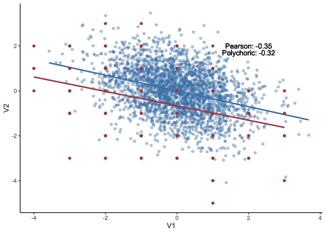
This method makes used of polychoric correlation as input, graphical LASSO as regularlization, and EBIC as model selection method. The polychoric correlation is a technique for estimating the correlation between two hypothesised normally distributed continuous latent variables, from two observed ordinal variables.
The figure below plot the relationships between two continous variables vs. relationships between two ordinal variables (using `floor` function). It appears that they did not deviate a lot given the values of pearson correlation (-.32) and polychoric correlation (-.3).
```{r}
dt <- as.data.frame(data[, 1:2])
dt_ordinal <- as.data.frame(floor(data[, 1:2]))

 # polychoric correlation
pearson_corr <- round(cor_auto(dt[, 1:2])[1, 2], 2)
polychoric_corr <- round(cor_auto(floor(data[, 1:2]))[1, 2], 2)
ggplot(dt) +
  geom_point(aes(x = V1, y = V2), data = dt, color = mycolors[1], alpha = .4) +
  geom_smooth(aes(x = V1, y = V2), data = dt, color = mycolors[1], method = "lm", se = FALSE) +
  geom_point(aes(x = V1, y = V2), data = dt_ordinal, color = mycolors[2]) +
  geom_smooth(aes(x = V1, y = V2), data = dt_ordinal, color = mycolors[2], method = "lm", se = FALSE) +
  geom_text(aes(x = 2, y = 2, label = paste0("Pearson: ", pearson_corr))) +
  geom_text(aes(x = 2, y = 1.7, label = paste0("Polychoric: ", polychoric_corr))) +
  theme_classic()
```
`EBICtuning <- 0.5` sets up the hyperparameter ($\gamma$) as .5 that controls how much the EBIC prefers simpler models (fewer edges), which by default is .5.
$$
\text{EBIC} =-2L+\log(N)+4\gamma \log(P)
$$
$$
\text{AIC} = -2L + 2P
$$
$$
\text{BIC} = -2L + P\log(N)
$$
Another important setting is the tuning parameter ($\lambda$) of EBICglasso that controls the sparsity level in the penalized likelihood function as:
$$
\log \det(\boldsymbol{K}) - \text{trace}(\boldsymbol{SK})-\lambda \Sigma|\kappa_{ij}|
$$
where $\boldsymbol{S}$ represents the sample variance-covariance matrix and $\boldsymbol{K}$ represents the precision matrix that *lasso* aims to estimate.
Overall, the regularization limits the sum of absolute partial correlation coefficients.
`sampleSize="pairwise_average"` will set the sample size to the average of sample sizes used for each individual correlation in `EBICglasso`.
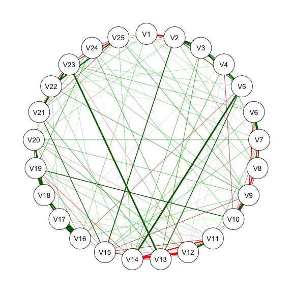
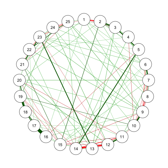
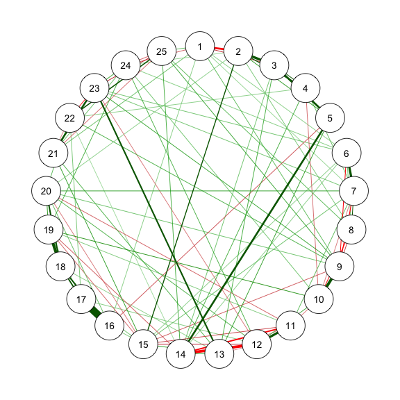
@fig-bfi is the estimated network structure with BFI-25 data.
```{r}
#| code-fold: show
#| code-summary: "Method 1: EBICglasso"
#| fig-width: 3
#| fig-height: 3
#| label: fig-bfi
#| fig-cap: "Method 1: Network Plot for BFI-25 with EBICglasso"
library("qgraph")
library("bootnet")
sampleAdjust  <-  "pairwise_average"
EBICtuning <- 0.5
transformation <- "polychoric/categorical" # EBICglasso use cor_auto
res_m1 <- estimateNetwork(data, # input as polychoric correlation
                          default = "EBICglasso",
                          sampleSize = sampleAdjust,
                          tuning = EBICtuning,
                          corMethod = ifelse(transformation == "polychoric/categorical",
                                             "cor_auto",
                                             "cor"))

estnet_m1 <- res_m1$graph
summary(res_m1)
str(res_m1$results)
EBIC = mean(res_m1$results$ebic) # EBIC of the final model
(AIC = EBIC - 2 * log(nrow(data))) # AIC =  52287.32
qgraph(estnet_m1)
```
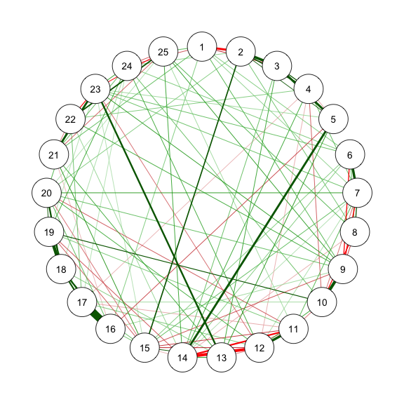
### Method 2 - ggmModSelect in bootnet
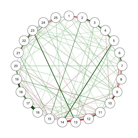
The *ggmModSelect* algorithm is a non-regularized method.
```{r}
#| code-fold: show
#| code-summary: "Method 2: ggmModSelect"
#| fig-width: 3
#| fig-height: 3
#| label: fig-m2_1
#| cache: true
#| fig-cap: "Method 2.1: Network Plot for BFI-25 with ggmModSelect and Stepwise"
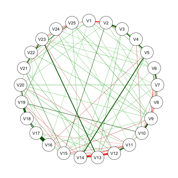
# With stepwise
res_m2_1 <- estimateNetwork(data, default = "ggmModSelect",
                           sampleSize = sampleAdjust, stepwise = TRUE,
                           tuning = EBICtuning,
                           corMethod = ifelse(transformation == "polychoric/categorical",
                                              "cor_auto",
                                              "cor"))

estnet_m2_1 <- res_m2_1$graph
qgraph(estnet_m2_1)
```
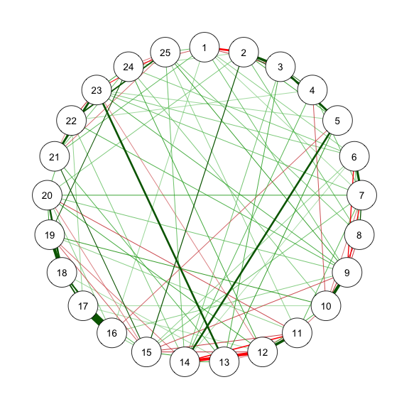
```{r}
#| code-fold: show
#| code-summary: "Method 2: ggmModSelect"
#| fig-width: 3
#| fig-height: 3
#| label: fig-m2_2
#| fig-cap: "Method 2.1: Network Plot for BFI-25 with ggmModSelect and No Stepwise"
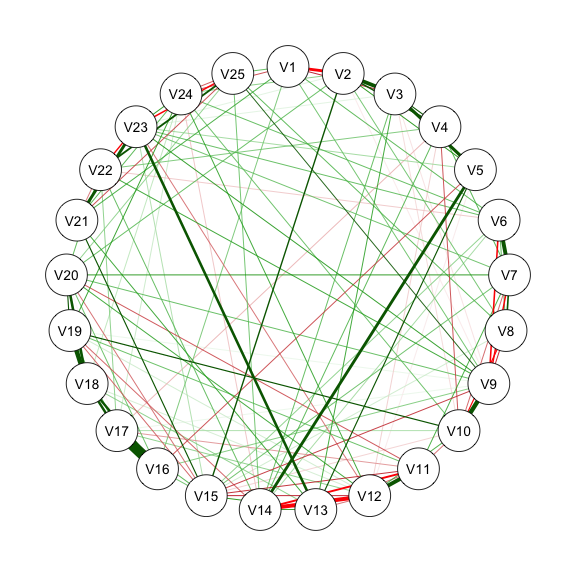
# Without stepwise
res_m2_2 <- estimateNetwork(data, default = "ggmModSelect",
                           sampleSize = sampleAdjust, stepwise = FALSE,
                           tuning = EBICtuning,
                           corMethod = ifelse(transformation == "polychoric/categorical",
                                              "cor_auto",
                                              "cor"))
estnet_m2_2 <- res_m2_2$graph
qgraph(estnet_m2_2)
```
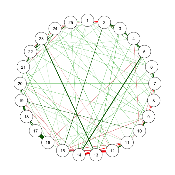
### Method 3 - FIML in psychonetrics
```{r}
#| code-fold: show
#| code-summary: "Method 3: FIML"
#| fig-width: 3
#| fig-height: 3
#| label: fig-m3_1
#| cache: true
#| fig-cap: "Method 3: Network Plot for BFI-25 with FIML and Prue"
library(psychonetrics)
library(magrittr)
# With stepwise
res_m3_1 <- ggm(data, estimator = "FIML", standardize = "z") %>%
  prune(alpha = .01, recursive = FALSE)

estnet_m3_1 <- getmatrix(res_m3_1, "omega")
fit(res_m3_1)
qgraph(estnet_m3_1)
```
```{r}
#| code-fold: show
#| code-summary: "Method 3: FIML"
#| fig-width: 3
#| fig-height: 3
#| label: fig-m3_2
#| cache: true
#| fig-cap: "Method 3: Network Plot for BFI-25 with FIML and Stepup"
# With stepwise
res_m3_2 <- ggm(data, estimator = "FIML", standardize = "z") %>%
  prune(alpha = .01, recursive = FALSE) |>
  stepup(alpha = .01)

estnet_m3_2 <- getmatrix(res_m3_2, "omega")

qgraph(estnet_m3_2)
```
### Method 4 - WLS in psychonetrics
```{r}
#| code-fold: show
#| code-summary: "Method 4: WLS"
#| fig-width: 3
#| fig-height: 3
#| label: fig-m4_1
#| cache: true
#| fig-cap: "Method 4: Network Plot for BFI-25 with WLS and prune"
# With stepwise
res_m4_1 <- ggm(data, estimator = "WLS", standardize = "z") %>%
  prune(alpha = .01, recursive = FALSE)

estnet_m4_1 <- getmatrix(res_m4_1, "omega")

qgraph(estnet_m4_1)
```
```{r}
#| code-fold: show
#| code-summary: "Method 4: WLS"
#| fig-width: 3
#| fig-height: 3
#| label: fig-m4_2
#| cache: true
#| fig-cap: "Method 4: Network Plot for BFI-25 with WLS, prune, and modelsearch"
res_m4_2 <- ggm(data, estimator = "WLS", standardize = "z") %>%
  prune(alpha = .01, recursive = FALSE) |>
  modelsearch(prunealpha = .01, addalpha = .01)

estnet_m4_2 <- getmatrix(res_m4_2, "omega")

qgraph(estnet_m4_2)
```
### Method 5 - mgm in mgm
`mgm` package is used for estimating mixed graphical models.
Node type can be "g" for Gaussian or "c" for categorical.
For continuous variables, set `level` to 1 and `type` to g.
```{r}
#| code-fold: show
#| code-summary: "Method 5: mgm"
#| fig-width: 3
#| fig-height: 3
#| label: fig-m5_1
#| cache: true
#| fig-cap: "Method 5: Network Plot for BFI-25 with mgm and CV"
library(mgm)
## mgm with CV
res_m5_1 <- mgm(na.omit(data), type = rep("g", ncol(data)), level = rep(1, ncol(data)),
           lambdaFolds = 20,
           lambdaSel = "CV", lambdaGam = EBICtuning,
           pbar = FALSE)
getmatrix_mgm <- function(res) {
  sign = ifelse(is.na(res$pairwise$signs), 1, res$pairwise$signs)
  sign * res$pairwise$wadj
}
estnet_m5_1 <- getmatrix_mgm(res_m5_1)
qgraph(estnet_m5_1)
```
```{r}
#| code-fold: show
#| code-summary: "Method 5: mgm"
#| fig-width: 3
#| fig-height: 3
#| label: fig-m5_2
#| cache: true
#| fig-cap: "Method 5: Network Plot for BFI-25 with mgm and EBIC"
## mgm with EBIC
res_m5_2 <- mgm(na.omit(data), type = rep("g", ncol(data)), level = rep(1, ncol(data)),
           lambdaFolds = 20,
           lambdaSel = "EBIC", lambdaGam = EBICtuning,
           pbar = FALSE)
estnet_m5_2 <- getmatrix_mgm(res_m5_2)
qgraph(estnet_m5_2)
```
### Method 6 - BGGM in BGGM
```{r}
#| code-fold: show
#| code-summary: "Method 6: BGGM"
#| fig-width: 3
#| fig-height: 3
#| label: fig-m6_1
#| fig-cap: "Method 6: Network Plot for BFI-25 with BGGM and explore"
res_m6_1 <- BGGM::explore(data, type = "continuous") |>
  BGGM:::select.explore(BF_cut = 3)
estnet_m6_1 <- res_m6_1$pcor_mat_zero
qgraph(estnet_m6_1)
```
```{r}
#| code-fold: show
#| code-summary: "Method 6: BGGM"
#| fig-width: 3
#| fig-height: 3
#| label: fig-m6_2
#| fig-cap: "Method 6: Network Plot for BFI-25 with BGGM and estimate"
res_m6_2 <- BGGM::explore(data, type = "continuous") |>
  BGGM:::select.estimate(cred = 0.95)
estnet_m6_2 <- res_m6_2$pcor_adj
qgraph(estnet_m6_2)
```
:::
## Performance Comparison
```{r}
performance <- function(network) {
  res_comparison <- comparison_metrics(real = as.matrix(bfi_truenetwork), est = as.matrix(network))
  c(
    sensitivity = res_comparison$sensitivity_full,
    specificity = res_comparison$specificity_full,
    precision = res_comparison$precision_full,

    abs_corr = res_comparison$abs_cor_true_edges_full, # The Pearson correlation between the absolute edge weights
    bias = res_comparison$bias_full, # The average absolute deviation
    bias_true = res_comparison$bias_true_edges_full # The average absolute deviation between the true edge weight and the estimated edge weight
  )
}
```
```{r}
performance_compr <- Reduce(rbind, lapply(list(estnet_m1, estnet_m2_1, estnet_m2_2,
                                               estnet_m3_1, estnet_m3_2,
                                               estnet_m4_1, estnet_m4_2,
                                               estnet_m5_1, estnet_m5_2,
                                               estnet_m6_1, estnet_m6_2), performance))
rownames(performance_compr) <- c("EBICglasso", "ggmModSelect_stepwise", "ggmModSelect_nostepwise",
                                 "FIML_prune", "FIML_stepup",
                                 "WLS_prune", "WLS_prune_modelsearch",
                                 "mgm_CV", "mgm_EBIC",
                                 "BGGM_explore", "BGGM_estimate")
kableExtra::kable(performance_compr, digits = 3)
```
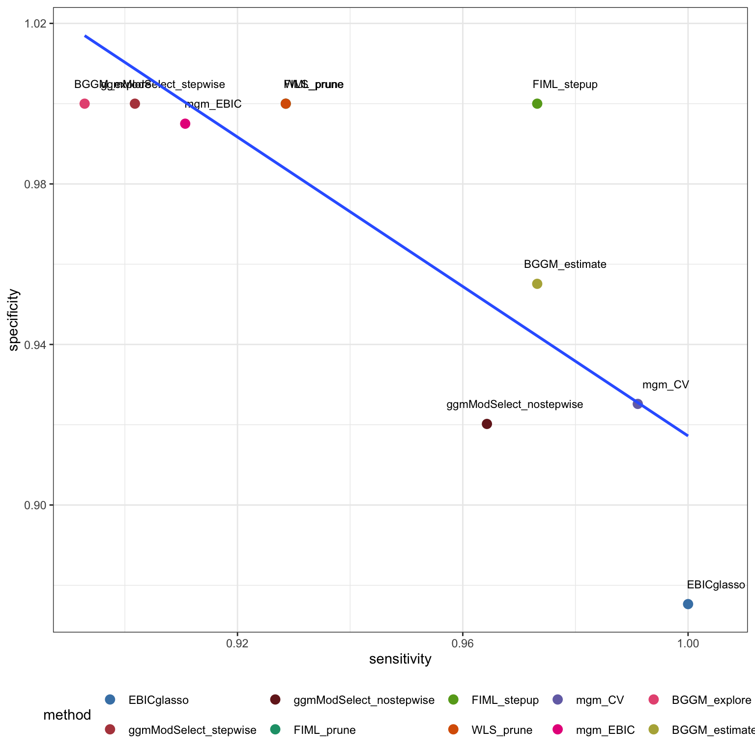
## Summary
```{r}
#| fig-width: 8
#| fig-height: 8
#| label: fig-summary01
#| fig-cap: "Specificity and Sensitivity Balance"
library(dplyr)
library(tidyr)
library(ggplot2)
mycolors = c("#4682B4", "#B4464B", "#752021",
             "#1B9E77", "#66A61E", "#D95F02", "#7570B3",
             "#E7298A", "#E75981", "#B4AF46", "#B4726A")
performance_tbl <- performance_compr |>
  as.data.frame() |>
  mutate(method = rownames(performance_compr)) |>
  mutate(method = factor(method, levels = rownames(performance_compr))) |>
  filter(
    method != "WLS_prune_modelsearch"
  )
ggplot(performance_tbl) +
  geom_point(aes(x = sensitivity, y = specificity, col = method), size = 3) +
  geom_text(aes(x = sensitivity, y = specificity, label = method), size = 3,
            nudge_x = .005, nudge_y = .005) +
  geom_smooth(aes(x = sensitivity, y = specificity), se = FALSE, method = lm) +
  theme_bw() +
  scale_color_manual(values = mycolors) +
  theme(legend.position = 'bottom')
```
`FLML_prune` and `BGGM_estimation` seem to perform best among all methods regarding balance between sensitivity and specificity of network weights.
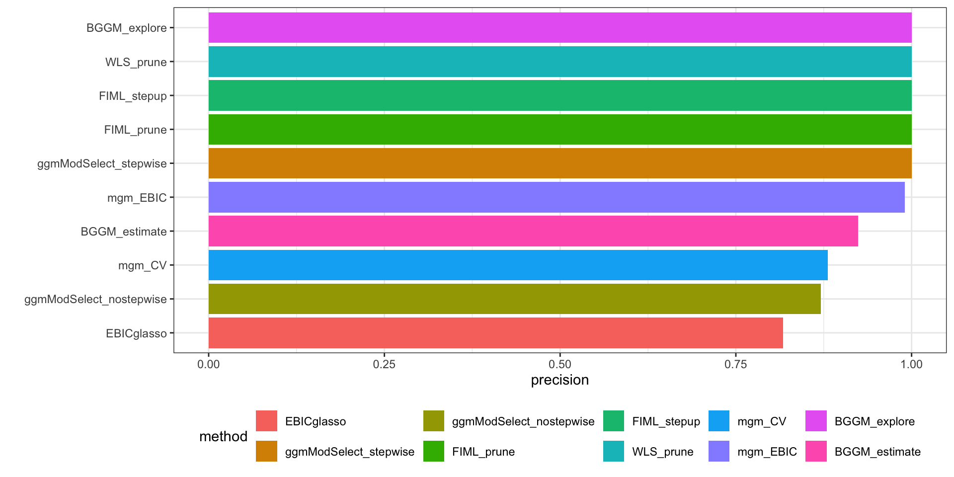
```{r}
#| fig-width: 10
#| fig-height: 5
#| label: fig-summary02
#| fig-cap: "Precision among all methods"
ggplot(performance_tbl) +
  geom_col(aes(y = forcats::fct_reorder(method, precision), x = precision, fill = method)) +
  theme_bw() +
  labs(y = "") +
  theme(legend.position = 'bottom')
```
`ggmMoSelect` with the stepwise procedure appears to have highest precision, followed by BGGM explore.