Psychometric Networks: Community = Clustering?

Overview

A friend of mine recently asked me one question about network community: in her recent research, a network without community defined has different estimation with the one with community define. Why this happens? In this blog, I try to dive a little deeper into community issues in psychometric network analysis. You can find my previous post on the estimation methods of network analysis - How To Choose Network Analysis Estimation For Application Research.

This blog instead aims to talk about varied aspects of community detection in psychometric network analysis, including the following questions:

1. What is “node community”?
2. Why we need communities of nodes in network analysis?
3. How communities are generated in the network?
4. How to identify those communities given a network?

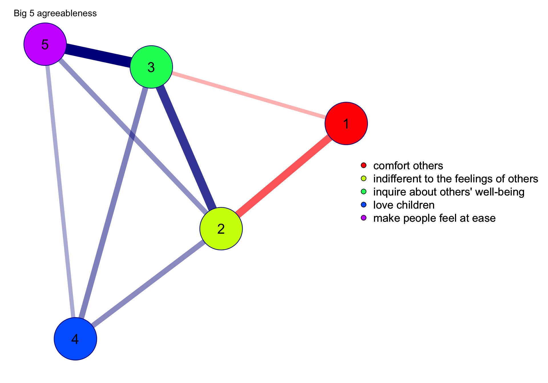
library(psychonetrics)
# Load bfi data from psych package:
library(psychTools)
# Also load dplyr for the pipe operator:
library(dplyr)


data(bfi)
# Let's take the agreeableness items, and gender:
ConsData <- bfi |> 
  select(A1:A5, gender) |> 
  na.omit() # Let's remove missingness (otherwise use Estimator = "FIML)

# Define variables:
vars <- names(ConsData)[1:5]

# Saturated estimation:
mod_saturated <- ggm(ConsData, vars = vars)

# Run the model:
mod_saturated <- mod_saturated |> runmodel()

# Labels:
labels <- c(
  "indifferent to the feelings of others",
  "inquire about others' well-being",
  "comfort others",
  "love children",
  "make people feel at ease")
# We can also fit an empty network:
mod0 <- ggm(ConsData, vars = vars, omega = "zero")

# Run the model:
mod0 <- mod0 |> runmodel()

# To automatically add along modification indices, we can use stepup:
mod1 <- mod0 |> stepup()

# Let's also prune all non-significant edges to finish:
mod1 <- mod1 |> prune()

qgraph::qgraph(getmatrix(mod1, "omega"),
               layout="spring",
               groups = labels,
               title = "Big 5 agreeableness",
               theme = "Borkulo",
               bg = rgb(red = 145, 
                        green = 203, 
                        blue = 215, 
                        alpha = .2196078431, 
                        maxColorValue = 255),
               transparency = TRUE)

1 Big problem in the network analysis

As said in Eiko’s post (E. Fried, 2016) and I cited here – authors sometimes over-interpret the network visualization of their data that some meaningful modules exist. This over-interpretation may have Type I error (mistakenly cluster nodes with actually weak connections in a community) or Type II error (fail to cluster nodes with strong connection into a community). In other words, researchers found that relying on visual inspection of network structure can not obtain reliable conclusion about which nodes should be clustered together and which ones should not be clustered, especially in a complicated network structure (say > 20 nodes).

Fried, E. (2016). R tutorial: How to identify communities of items in networks. In Psych Networks. https://psych-networks.com/r-tutorial-identify-communities-items-networks/

Identification of node clusters is not a new topic, which is typically called “Community Detection” in graph theory (Fortunato, 2010). This problem arises due to a phenomenon called “Community Structure”(Girvan & Newman, 2002) or “Clustering” was found in varied types of networks. This community structure has two characteristics:

1. Heterogeneity of node degree: nodes with high degree (more neighbors/ high betweenness) coexist with nodes with low degree.
2. Heterogeneity of edge strength: high concentrations of edges with certain “group” of nodes even though those “groups” are visual inspected.

Given this community structure, Community (or called clusters or modules) is defined as groups of nodes which probably share common properties and / or play similar roles within the graph (Fortunato, 2010). This is actually a very broad definition which does not answer what are “common properties” and “similar roles” in a network graph. The reason of this vagueness is because of variety of network in different areas.

Fortunato, S. (2010). Community detection in graphs. Physics Reports, 486(3), 75–174. https://doi.org/10.1016/j.physrep.2009.11.002

Zhang, J., & Liang, X. (2024). Evaluating general network scoring methods as alternatives to traditional factor scoring methods. https://doi.org/10.31234/osf.io/s3re6

Andersson, B., & Xin, T. (2021). Estimation of latent regression item response theory models using a second-order laplace approximation. Journal of Educational and Behavioral Statistics, 46(2), 244–265. https://doi.org/10.3102/1076998620945199

Yamaguchi, K., & Zhang, J. (2023). Fully gibbs sampling algorithms for bayesian variable selection in latent regression models. Journal of Educational Measurement, 60(2), 202–234. https://doi.org/10.1111/jedm.12348

For example, within a social network of one person, one individual is considered as node and his/her social relationship with other people as edges, then “communities” may be conceptualized as family, company, or any other social groups. The latent common causes of community in social network may be the shared emotional pattern constructed via the family education, close levels of cognitive abilities within same university/college/classroom, in or similar behavioral pattern under company policy. In protein-protein interaction networks, communities are likely to group proteins having the same specific function within the cell. In the graph of the World Wide Web, community may correspond to groups of web pages dealing with the same or related topics. The regression-based relationship between community and external factors has not been well developed to my knowledge, i.e., the relationship between depression community with age, education, and other disorders. Currently, community-level centrality-based network scores (Zhang & Liang, 2024) can be used as measurement of the community, which then can potentially be used as independent variables or outcome in a regression model. However, network scores are suffering from interpretability in psychometrics and relevant research on this topic is still sparse. Similar idea can be found in other psychometric modeling, such as latent regression model in latent variable modeling literature (Andersson & Xin, 2021; Yamaguchi & Zhang, 2023) or the structural model in structural equation modeling.

Back to the community conceptualization in psychological area, especially psychiatry, the community is usually associated with syndromes or comorbidity. According to Wikipedia, a syndrome is a set of medical signs and symptoms which are correlated with each other and often associated with a particular disease or disorder. Some psychological syndromes may present comorbidity of symptoms, which refers to simultaneous presence of two or more psychological symptoms in a same individual within a time frame (co-occurring, concurrent). In a earlier paper of Borsboom (2002), Borsboom took the DSM-IV (Diagnostic and Statistical Manual of Mental Disorders) as example and argued that “… Commodity appears to be, at least partially and in particular for mood, anxiety, and substance abuse disorders, encoded in the structure of the diagnostic criteria themselves” (Borsboom, 2002), but he did not link the “commodity” of a cluster of highly-connected symptoms to the statistical concept “community” in network graph. It is until the paper of Cramer et al. (2010), the symptom community as a local connectivity was considered as syndromes, while symptoms clusters are interconnected by individual symptoms (“bridge symptoms”) that form the boundaries between the various basic syndromes of psychiatric disorders (Goekoop & Goekoop, 2014). Goekoop & Goekoop (2014) also emphasized that the presence of bridge symptoms that connects symptom clusters (communities / syndromes) plays a key role that can be identified as potential targets for treatment.

Borsboom, D. (2002). The structure of the DSM. Archives of General Psychiatry, 59(6), 569–570.

Cramer, A. O. J., Waldorp, L. J., Maas, H. L. J. van der, & Borsboom, D. (2010). Comorbidity: A network perspective. Behavioral and Brain Sciences, 33(2-3), 137–150. https://doi.org/10.1017/S0140525X09991567

Goekoop, R., & Goekoop, J. G. (2014). A network view on psychiatric disorders: Network clusters of symptoms as elementary syndromes of psychopathology. PLOS ONE, 9(11), e112734. https://doi.org/10.1371/journal.pone.0112734

2 Identify Community

There are two ways of defining communities in psychometric network: the exploratory method and the confirmatory method. The exploratory method has a long root in the graphical theory (e.g., exploratory graphical analysis). Exploratory graphical analysis (EGA) makes use of community detection algorithm to detect potential communities in a complex network structure.

In psychometric literature, however, confirmatory network analysis has become more and more popular (Du et al., 2024). Although the value of exploratory research remains indisputable, the field of psychology is facing an increasing demand for theory- and hypothesis-testing research, which serves to confirm, refute, or refine existing theories (Du et al., 2024; E. I. Fried, 2020). For example, many “communities” should correspond to theoretical constructs in psychology or education settings. That is, psychopathology syndrome mentioned above must have one precise definition in DSM-V for the clinician references, so relevant indicators (nodes) then should be grouped into one community prior to the network analysis. The network modeling with pre-defined communities is called confirmatory network analysis. As said by Hevey (2018), I cited here, “… much of the research in psychological networks has been based on exploratory data analyses to generate networks; there is a need to progress towards confirmatory network modelling wherein hypotheses about network structure are formally tested.”

Du, X., Skjerdingstad, N., Freichel, R., Ebrahimi, O. V., Hoekstra, R. H. A., & Epskamp, S. (2024). Moving from exploratory to confirmatory network analysis: An evaluation of SEM fit indices and cutoff values in network psychometrics. https://doi.org/10.31234/osf.io/d76ab

Fried, E. I. (2020). Lack of theory building and testing impedes progress in the factor and network literature. Psychological Inquiry, 31(4), 271–288. https://doi.org/10.1080/1047840X.2020.1853461

Hevey, D. (2018). Network analysis: A brief overview and tutorial. Health Psychology and Behavioral Medicine, 6(1), 301–328. https://doi.org/10.1080/21642850.2018.1521283

E. I. Fried (2020) mentioned some challenges in psychology research and argued that the core issues—latent theories, weak theories, and conflating theoretical and statistical models—are common and harmful, facilitate invalid inferences, and stand in the way of theory failure and reform.

1. The statistical and theoretical models are conflated without concrete evidence of the existence of psychological constructs.
2. Unclear theoretical grounds and unclear what the theory actually explains/predicts.

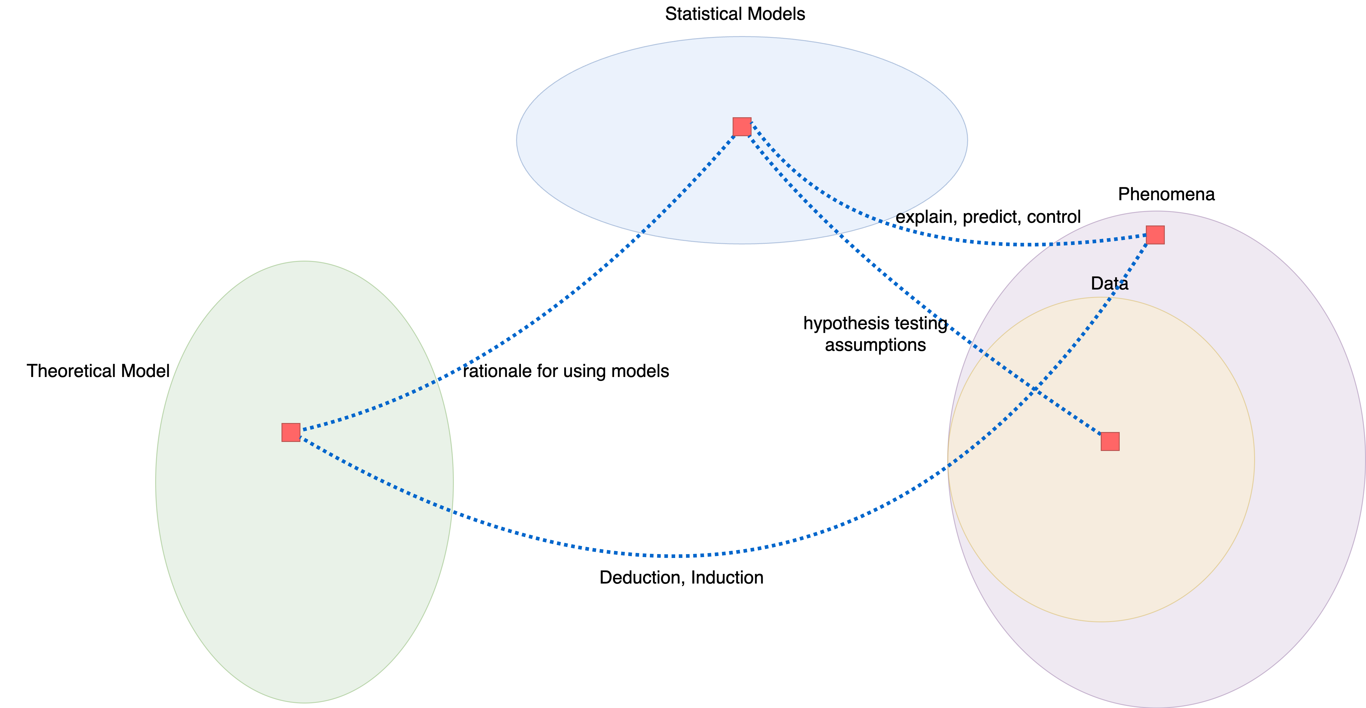
Theories are those tools can explain, predict, control phenomena. They are also in one point between strong to weak given to what degree they can explain, predict, and control phenomena. Typically, theorectical model is related to the date generation process—how data is generated, which is unknown in prior. We can link theory to data by using statistical modeling that impose assumptions on the data. However, the statistical models themselves can not be used to measure how strong or weak the theory is.

Relationships among theory, statistical model, and data

2.1 Community Detection Algorithm

Numerous prior studies have compared different community detection methods in varied network structure (Gates et al., 2016; Yang et al., 2016). In the framework of latent factor analysis or psychometric network, Christensen et al. (2024) recently conducted a Monte-Carlo simulation study compared various node community detection algorithm. To interpret the results, Christensen et al. (2024) even created a Shiny App to interactive present the results.

Gates, K. M., Henry, T., Steinley, D., & Fair, D. A. (2016). A monte carlo evaluation of weighted community detection algorithms. Frontiers in Neuroinformatics, 10. https://doi.org/10.3389/fninf.2016.00045

Yang, Z., Algesheimer, R., & Tessone, C. J. (2016). A comparative analysis of community detection algorithms on artificial networks. Scientific Reports, 6(1), 30750. https://doi.org/10.1038/srep30750

Christensen, A. P., Garrido, L. E., Guerra-Peña, K., & Golino, H. (2024). Comparing community detection algorithms in psychometric networks: A monte carlo simulation. Behavior Research Methods, 56(3), 1485–1505. https://doi.org/10.3758/s13428-023-02106-4

Table 1: Different types of community detection algorithms

Algorithm	Feature
Walktrap (Pons & Latapy, 2006)	random walks
Infomap (Rosvall & Bergstrom, 2008)	random walks
Fast-greedy (Clauset et al., 2004)	hierarchical clustering; modularity-based
Louvian (Blondel et al., 2008)	hierarchical clustering; modularity-based
Leading Eigenvalue (Newman, 2006)	eigenvalue
Label Propagation (Raghavan et al., 2007)	non-parametric
Spinglass (Reichardt & Bornholdt, 2006)	non-parametric
Edge Betweenness (Girvan & Newman, 2002)	non-parametric
Triangulated Maximally Filtered Graph (TMFG) (Massara et al., 2017)	score based
Parallel Analysis	EFA

Pons, P., & Latapy, M. (2006). Computing communities in large networks using random walks. Journal of Graph Algorithms and Applications, 10(22), 191–218. https://doi.org/10.7155/jgaa.00124

Rosvall, M., & Bergstrom, C. T. (2008). Maps of random walks on complex networks reveal community structure. Proceedings of the National Academy of Sciences, 105(4), 1118–1123. https://doi.org/10.1073/pnas.0706851105

Clauset, A., Newman, M. E. J., & Moore, C. (2004). Finding community structure in very large networks. Physical Review E, 70(6), 066111. https://doi.org/10.1103/PhysRevE.70.066111

Blondel, V. D., Guillaume, J.-L., Lambiotte, R., & Lefebvre, E. (2008). Fast unfolding of communities in large networks. Journal of Statistical Mechanics: Theory and Experiment, 2008(10), P10008. https://doi.org/10.1088/1742-5468/2008/10/P10008

Newman, M. E. J. (2006). Modularity and community structure in networks. Proceedings of the National Academy of Sciences, 103(23), 8577–8582. https://doi.org/10.1073/pnas.0601602103

Raghavan, U. N., Albert, R., & Kumara, S. (2007). Near linear time algorithm to detect community structures in large-scale networks. Physical Review E, 76(3), 036106. https://doi.org/10.1103/PhysRevE.76.036106

Reichardt, J., & Bornholdt, S. (2006). Statistical mechanics of community detection. Physical Review E, 74(1), 016110. https://doi.org/10.1103/PhysRevE.74.016110

Girvan, M., & Newman, M. E. J. (2002). Community structure in social and biological networks. Proceedings of the National Academy of Sciences, 99(12), 7821–7826. https://doi.org/10.1073/pnas.122653799

Massara, G. P., Di Matteo, T., & Aste, T. (2017). Network filtering for big data: Triangulated maximally filtered graph. Journal of Complex Networks, 5(2), 161–178. https://doi.org/10.1093/comnet/cnw015

Table 1 shows the list of community detection algorithms and their features. In the framework of psychometric assessment (< 50 nodes, balanced item number per factor), the best-performing algorithms are GLASSO with unidimentional adjustment, Louvian, Fast-greedy, Walktrap, and parallel analysis. The evaluation criteria include:

1. The percentage of correct number of factors (PC)
2. Mean absolute error (MAE; the average absolute deviation away from the correct number of factors)
3. Mean bias error (MBE; the average deviation away from the correct number of factors)

Assume N is the total number of simulated sample date sets (Replication), K is the population number of factors/communities, and \hat{K} is the estimated number of factors/communities. \mathbb{I}(\cdot) is the indicator function so that \mathbb{I}(\hat{K}, K) = 1 if \hat{K} = K and \mathbb{I}(\hat{K}, K) = 0 otherwise. The three evaluation criteria are defined as:

\mathrm{PC} = \frac{1}{N} \sum_{i=1}^{N} \mathbb{I}(\hat{K}_i, K_i)

\mathrm{MAE} = \frac{1}{N} \sum_{i=1}^{N} |\hat{K}_i - K_i|

\mathrm{MBE} = \frac{1}{N} \sum_{i=1}^{N} (\hat{K}_i - K_i)

## K is a vector of population number of factors with the length of number replications
## K_hat is a vector of estimate number of factors with the length of number replications
cal_pc <- function(K, K_hat) {
  N <- length(K)
  pc <- sum(K_hat == K) / N
  return(pc)
}
cal_mae <- function(K, K_hat) {
  N <- length(K)
  mae <- sum(abs(K_hat - K)) / N
  return(mae)
}
cal_mbe <- function(K, K_hat) {
  N <- length(K)
  mbe <- sum(K_hat - K) / N
  return(mbe)
}

3 Example: Accuracy and Stability for Fast Greedy and Walktrap

For illustration, we can examine the differences in accuracy and stability between the fast-greedy method and the walktrap method due to the sampling error. The sample data is the Big-five questionnaire dataset (N=2800). The bootstrapping resampling method with 100 replications and 10% total sample size is used for the analysis.

For evaluation criteria, the standardized deviation (SD) for two methods was used to examine the stability; PC, MAE, MBE for two methods were used to examine the accuracy.

library(igraph) # For community detection
library(foreach) # For parallel computing
library(doParallel) # For core registration

# Load bfi data from psych package:
Data <- bfi |> 
  select(A1:A5, C1:C5, E1:E5, N1:N5, O1:O5) |> 
  na.omit()

ten_perc_N = floor(nrow(Data) / 10) # Number of cases for 10% sample size
N_replications <- 100 # Number of bootstrapping resampling

# Function to get the number of communities by fast-greedy and walktrap
get_resampling_community_n <- \(dat, i, size) {
  set.seed(1234 + i)
  sampled_cases <- dat[sample(x = 1:nrow(dat), size = size), ]
  # Define variables:
  vars <- names(dat)
  
  # Saturated estimation:
  mod_sparsed <- ggm(sampled_cases, vars = vars) |> runmodel()  |>  stepup() |>  prune()
  
  ## Get edge weights
  omega_mat <- getmatrix(mod_sparsed, "omega")
  
  ## Convert to igraph object from adjcent matrix
  ggm_igraph <- graph_from_adjacency_matrix(adjmatrix = abs(omega_mat), 
                                            weighted = TRUE, 
                                            mode = "undirected")
  
  ## Apply Walktrap / Fast Greedy Community Detection Algoritm 
  ggm_wt <- cluster_walktrap(ggm_igraph)
  ggm_fg <- cluster_fast_greedy(ggm_igraph)
  
  ## Get number of detected communities 
  return(
    c(K_wt = length(ggm_wt), 
      K_fg = length(ggm_fg),
      size = size, 
      seed = (1234 + i))
  )
}

cl <- makePSOCKcluster(detectCores() - 1)
registerDoParallel(cl)
res <- foreach(i = 1:N_replications, 
               .packages = c("psychonetrics", "igraph"),
               .combine = "rbind") %dopar% 
  get_resampling_community_n(dat = Data, i = i, size = ten_perc_N)
stopCluster(cl)

K_wt <- res[,1]
K_fg <- res[,2]
report <- data.frame(
  Algorithm = c("Walktrap", "Fast-Greedy"),
  PC = sapply(list(K_wt, K_fg), \(x) cal_pc(x, rep(5, length(x))) ),
  MAE = sapply(list(K_wt, K_fg), \(x) cal_mae(x, rep(5, length(x))) ),
  MBE = sapply(list(K_wt, K_fg), \(x) cal_mbe(x, rep(5, length(x))) )
)
kableExtra::kable(report)

Algorithm	PC	MAE	MBE
Walktrap	0.35	0.97	-0.71
Fast-Greedy	0.61	0.41	-0.17

summary_tbl <- data.frame(
  Algorithm = c("Walktrap", "Fast-Greedy"),
  Min = sapply(list(K_wt, K_fg), min),
  Max = sapply(list(K_wt, K_fg), max),
  Mean = sapply(list(K_wt, K_fg), mean),
  SD = sapply(list(K_wt, K_fg), sd)
)
kableExtra::kable(summary_tbl)

Algorithm	Min	Max	Mean	SD
Walktrap	4	9	5.71	1.1307904
Fast-Greedy	4	7	5.17	0.6521913

Interpretation

Overall, the fast-greedy method performs better than the walktrap method given its higher value of PC and lower absolute values of MAE and MBE across 100 bootstrapping re-sampling iterations with the \frac{1}{10} sample size. The fast-greedy is also more stable than the walktrap given smaller variability (\mathrm{SD_{FG}}=.65; \mathrm{SD_{WT}}=1.13).

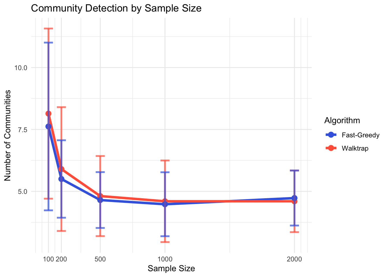
3.1 Sample Size Effect on Community Detection

We can further examine the effect of sample size on the community detection. The sample sizes are 100, 200, 500, 1000, and 2000. The bootstrapping resampling method with 100 replications is used for variability in each condition.

cl <- makePSOCKcluster(detectCores() - 1)
registerDoParallel(cl)
res_byN <- foreach(N = c(100, 200, 500, 1000, 2000), 
        .packages = c("psychonetrics", "igraph"),
        .combine = "rbind") %:%
  foreach(i = 1:N_replications, .combine = "rbind") %dopar%
  get_resampling_community_n(dat = Data, i = i, size = N)
stopCluster(cl)

library(tidyverse)
res_byN_tbl <- as.data.frame(res_byN) 

res_byN_smy <- res_byN_tbl |> 
  group_by(size) |> 
  summarise(
    wt_mean = mean(K_wt),
    fg_mean = mean(K_fg),
    wt_sd = sd(K_wt),
    fg_sd = sd(K_fg)
  )

library(ggplot2)
library(tidyr)
res_byN_smy |> 
  tidyr::pivot_longer(cols = -size, names_to = "Algorithm", values_to = "K") |>
  tidyr::separate(Algorithm, into = c("Algorithm", "Stat"), sep = "_") |> 
  tidyr::pivot_wider(names_from = Stat, values_from = K) |> 
  ggplot(aes(x = size, color = Algorithm, group = Algorithm)) +
  geom_path(aes(y = mean), linewidth = 1.5) +
  geom_point(aes(y = mean), size = 3) +
  geom_errorbar(aes(ymin = mean - 1.96*sd, ymax = mean + 1.96*sd), 
                width = 70, linewidth = 1.1, alpha = .7) +
  labs(title = "Community Detection by Sample Size",
       x = "Sample Size",
       y = "Number of Communities") +
  scale_color_manual(values = c("royalblue", "tomato"), labels = c("Fast-Greedy", "Walktrap")) +
  scale_x_continuous(breaks = c(100, 200, 500, 1000, 2000)) +
  theme_minimal()

Figure 1: Community Detection by Sample Size

As shown in Figure 1, for both methods, as sample size gets larger, the number of communities detected by both methods tends to align with the theoretical number of communities, K = 5. From N = 100 to N = 200 has strong increase in the accuracy of the number of communities detected, while from N = 200 to N = 500 has moderate improvement in the number of communities detected. After N = 500, the number of communities detected is stable.