---
title: "Reliability and Replicability of the Psychological Network Analysis"
date: 'May 3 2024'
image: "reliability-of-network-psychometrics_files/figure-html/unnamed-chunk-5-1.png"
categories:
- R
- Bayesian
- Tutorial
- Network Analysis
execute:
eval: true
echo: true
warning: false
fig-align: center
format:
html:
code-fold: true
code-summary: 'Click to see the code'
toc-location: right
toc-depth: 2
toc-expand: true
bibliography: references.bib
---
# Empirical study 1: PTSD networks
This study examines the reliability and replicability of the network structure of PTSD symptoms in a large sample of trauma-exposed individuals.
Fried et al. (2018) shared their correlation matrices, model output, and code in the [Supplementary Materials](https://doi.org/10.1080/00273171.2019.1616526) and encouraged reanalysis of the data for further replicability research.
This data sets were reanalyzed by [@forbesQuantifyingReliabilityReplicability2021].
## Research Plan
First, the PTSD network structure will be estimated through three models:
- **Model 1**: Gaussian graphical models (GGMs) derived from polychoric correlations using fused graphical lasso selecting tuning parameters using k-fold cross-validation first.
- **Model 2**: GGM using FIML in *psychonetrics* (`FLML_prune`)
- **Model 3**: Bayesian GGM using `BGGM_estimation`, which have best performance in sensitivity and specificity.
Second, the parameter estimation and network characteristics will be carefully screened and reviewed.
- Network characteristics across waves
1. Node strength (NS_max, NS_min)
2. Number of total possible edges (Num_total_edges)
3. Number of estimated (non-zero) edges (Num_nonzero_edges)
4. Connectivity -- percentage of edges that are non-zero (Connectivity)
5. Number of zero edges (Num_zero_edges)
6. Number of positive edges (Num_positive_edges)
7. Number of negative edges (Num_negative_edges)
- Bootstrap and NCT results
1. Edges bootstrapped CIs
2. Strength centrality bootstrapped CIs
3. NCT omnibus test
```{r}
##Network characteristics
network_char <- function(network) {
  graph <- network$graph
  #edge lists
  edges <- graph[upper.tri(graph)]

  #node strength
  strengthT1<-centrality(graph)$OutDegree
  NS_sum <- sum(strengthT1)
  NS_max <- max(strengthT1)
  NS_min <- min(strengthT1)

  # Number of total possible edges
  totalT1 <- length(edges)
  Num_total_edges <- totalT1

  # Number of estimated edges:
  nedges<- sum(edges!=0)
  Num_nonzero_edges <- nedges

  #Connectivity
  connectT1<-round(nedges/totalT1 * 100, 1)
  Connectivity <- connectT1

  #Number of zero edges
  n0edges<- sum(edges==0)
  Num_zero_edges <- n0edges

  #Number of positive edges
  nposedges<- sum(edges>0)
  Num_positive_edges <- nposedges

  #Number of negative edges
  nnegedges<- sum(edges<0)
  Num_negative_edges <- nnegedges

  #Bootstrap confidence intervals
  boot1a <- bootnet(network, nCores = 6, nBoots = 1000)
  boot1a_summary <- summary(boot1a, type = "CIs", nCores = 6)
  Num_nonzero_edges_bootstrap <- sum(sign(boot1a_summary$CIlower) == sign(boot1a_summary$CIupper) & sign(boot1a_summary$CIlower) != 0)
  Num_positive_edges_bootstrap <- sum(sign(boot1a_summary$CIlower) == sign(boot1a_summary$CIupper) & sign(boot1a_summary$CIlower) == 1)

  c(NS_sum = round(NS_sum, 2),
    NS_max = round(NS_max, 2),
    NS_min = round(NS_min, 2),
    Connectivity= Connectivity,
    Num_total_edges= Num_total_edges,
    Num_nonzero_edges= Num_nonzero_edges,
    Num_nonzero_edges_bootstrap = Num_nonzero_edges_bootstrap,
    Num_zero_edges= Num_zero_edges,
    Num_positive_edges= Num_positive_edges,
    Num_positive_edges_bootstrap= Num_positive_edges_bootstrap,
    Num_negative_edges= Num_negative_edges)
}
```
## Data Information
"*The primary analyses were based on a subset of community participants from a larger longitudinal study. Analyses included 403 participants who completed questions online regarding depression and anxiety symptoms two times one week apart.* [@forbesQuantifyingReliabilityReplicability2021]"
| Node label | Symptom |
|------------|-------------------------------------------------------------------------|
| PHQ1 | Little interest or pleasure in doing things |
| PHQ2 | Feeling down, depressed, or hopeless |
| PHQ3 | Trouble falling or staying asleep, or sleeping too much |
| PHQ4 | Feeling tired or having little energy |
| PHQ5 | Poor appetite or overeating |
| PHQ6 | Feeling bad about yourself — or that you are a failure or have let yourself or your family down |
| PHQ7 | Trouble concentrating on things, such as reading the newspaper or watching television |
| PHQ8 | Moving or speaking so slowly that other people could have noticed? Or the opposite—being so fidgety or restless that you have been moving around a lot more than usual |
| PHQ9 | Thoughts that you would be better off dead or of hurting yourself in some way |
| GAD1 | Feeling nervous, anxious, or on edge |
| GAD2 | Not being able to stop or control worrying |
| GAD3 | Worrying too much about different things |
| GAD4 | Trouble relaxing |
| GAD5 | Being so restless that it’s hard to sit still |
| GAD6 | Becoming easily annoyed or irritable |
| GAD7 | Feeling afraid as if something awful might happen |
## Data Analysis
To replicate the same analysis as @forbesQuantifyingReliabilityReplicability2021, we used the raw data from their OSF project (<https://osf.io/6fk3v/>)
```{r}
#| code-summary: "List the files in the OSF project of (Forbes et al., 2021)"
library(osfr)
forbes2018 <- project <- osf_retrieve_node("https://osf.io/6fk3v/")
osf_ls_files(forbes2018)
```
Download the two-wave data set (`time1and2data_wide.csv`).
```{r}
#| eval: false
#| code-summary: "Download the time1and2data_wide.csv"
forbes2018_files <- osf_ls_files(forbes2018)
osf_download(forbes2018_files[7, ], path = "PTSD_network/")
osf_download(forbes2018_files[4, ], path = "PTSD_network/")
```
There are 403 participants with 40 variables and 1 ID.
```{r}
#| code-summary: "Read in the data set"
# Set the random seed:
set.seed(123)

# Load time1 dataset:
time1and2data <- read.csv("PTSD_network/time1and2data_wide.csv", header=FALSE)
time1and2data<-as.data.frame(time1and2data)
time1data<- time1and2data[c(2:17)]
time1data<-as.data.frame(time1data)
labels_time1and2data <- c("PHQ1","PHQ2","PHQ3","PHQ4","PHQ5","PHQ6","PHQ7",
                       "PHQ8","PHQ9","GAD1","GAD2","GAD3","GAD4","GAD5",
                       "GAD6","GAD7")
groups_time1and2data <- c(rep("Depression", 9), rep("Anxiety", 7))
time2data<- time1and2data[c(18:33)]
time2data<-as.data.frame(time2data)
colnames(time2data) <- colnames(time1data) <- labels_time1and2data
Labels<- c("interest", "feel down", "sleep", "tired", "appetite", "self-esteem",
            "concentration", "psychomotor", "suicidality", "feel nervous",
            "uncontrollable worry", "worry a lot", "trouble relax", "restless",
            "irritable", "something awful")
time1dep<-time1data[c(1:9)]
time1anx<-time1data[c(10:16)]
time2dep<-time2data[c(1:9)]
time2anx<-time2data[c(10:16)]
```
The Patient Health Questionnaire (PHQ-9; Kroenke, Spitzer & Williams, 2001) is a 9-item measure of depression symptoms with cutoff scores that indicate clinically significant levels of major depression.
The Brief Measure for Assessing Generalized Anxiety Disorder (GAD-7; Spitzer, Kroenke, Williams & Lowe, 2006) is a 7-item measure of anxiety symptoms with cutoff scores that indicate clinically significant levels of generalized anxiety (Spitzer et al., 2006).
Both questionnaires have the scale options (0 – “Not at all,” 1 – “Several days,” 2 – “More than half the days,”, 3 – “Nearly every day”).
```{r}
#| code-summary: "Time 1 dataset"
library(gt)
library(DT)
datatable(time1data)
```
::: panel-tabset
### Model 1: EBICglasso
Model 1 — The depression and anxiety symptom networks were estimated as Gaussian graphical models (GGM) separately at each wave using graphical LASSO regularization with EBIC.
The package is `bootnet::estimateNetwork` with "EBICglasso".
This is same as using `qgraph::EBICglasso()`.
The default setting of this function is converting input data into polychoric correlation matrix.
```{r}
#| code-summary: "Visualize strength centrality for wave 1 and 2"
library(bootnet)
library(qgraph)
mycolors = c("#4682B4", "#B4464B", "#752021",
"#1B9E77", "#66A61E", "#D95F02", "#7570B3",
"#E7298A", "#E75981", "#B4AF46", "#B4726A")
##Estimate GGM networks
network1 <- estimateNetwork(time1data, default="EBICglasso")
network2 <- estimateNetwork(time2data, default="EBICglasso")
layout(t(1:1))
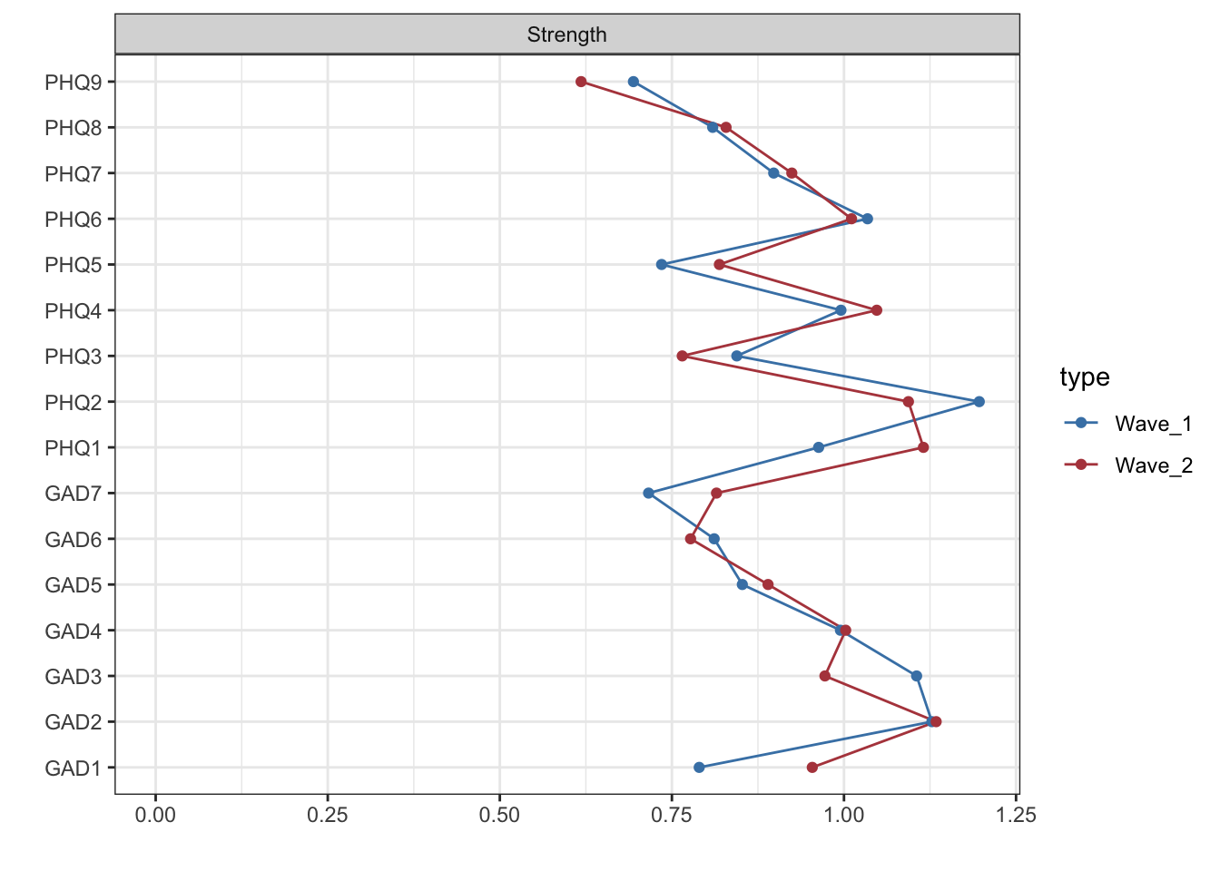
centw1w2 <- centralityPlot(list(Wave_1 = network1, Wave_2 = network2),
labels=labels_time1and2data, verbose = FALSE,
print = F)
centw1w2 + scale_color_manual(values = mycolors)
```
```{r}
#| code-summary: "Visualize network structure for wave 1 and 2"
#| fig-width: 9
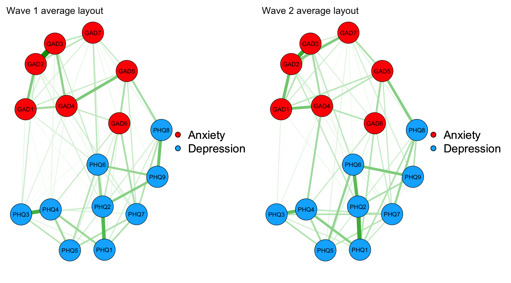
L <- averageLayout(network1, network2)
#Plot networks with average layout and edges comparable in weight
maxIsing<-max(c(network1$graph, network2$graph))
layout(t(1:2))
network1plot_average <- qgraph(network1$graph, layout=L, title="Wave 1 average layout", maximum=maxIsing, groups = groups_time1and2data)
network2plot_average <- qgraph(network2$graph, layout=L, title="Wave 2 average layout", maximum=maxIsing, groups = groups_time1and2data)
```
```{r network_characteristics}
#| code-summary: "Network characteristics for wave 1 and 2"
Networ_char_labes <- c(
  NS_sum = "Global strength (sum absolute edge weights)",
  NS_max = "Maximum strength",
  NS_min = "Minimum strength",
  Connectivity = "Connectivity (percentage of edges that are non-zero)",
  Num_total_edges = "Total number of possible edges",
  Num_nonzero_edges = "Number of non-zero edges",
  Num_nonzero_edges = "Number of boostrapped non-zero edges",
  Num_zero_edges = "Number of zero edges",
  Num_positive_edges = "Number of positive edges",
  Num_nonzero_edges = "Number of boostrapped positive edges",
  Num_negative_edges = "Number of negative edges"
)

if (file.exists("tables/network_char_tbl.csv")){
  network_char_tbl <- read.csv("tables/network_char_tbl.csv")
}else{
  network_char_tbl <- data.frame(
    `Network characteristics` = Networ_char_labes,
    Wave1 = network_char(network1),
    Wave2 = network_char(network2)
  )
  write.csv(network_char_tbl, file = "tables/network_char_tbl.csv", row.names = FALSE)
}
```
```{r}
#| echo: false
datatable(network_char_tbl)
```
```{r}
#| code-summary: "Most influential nodes for wave 1 and 2 based on node strength"
library(tidyverse)
centralityTable(list(Wave_1 = network1,
                     Wave_2 = network2)) |>
  dplyr::filter(measure == "Strength") |>
  group_by(type) |>
  dplyr::filter(value == max(value)) |>
  kableExtra::kable()
```
### Model 2: FIML with prune
```{r}
#| code-summary: "Esimate the network with psychonetrics"
library(psychonetrics)
network1_mod2 <- ggm(time1data, estimator = "FIML", standardize = "z") %>%
  prune(alpha = .01, recursive = FALSE)
network2_mod2 <- ggm(time2data, estimator = "FIML", standardize = "z") %>%
  prune(alpha = .01, recursive = FALSE)
network1_mod2_graph <- getmatrix(network1_mod2, "omega")
network2_mod2_graph <- getmatrix(network2_mod2, "omega")
```
```{r}
#| code-summary: "Visualize strength centrality for wave 1 and 2"
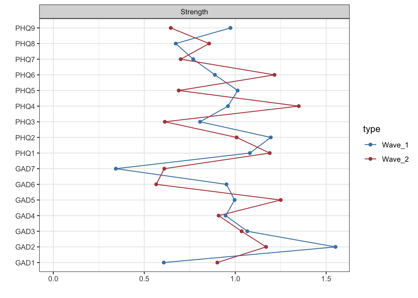
centw1w2_mod2 <- centralityPlot(list(Wave_1 = network1_mod2_graph, Wave_2 = network2_mod2_graph),
                           labels=labels_time1and2data, verbose = FALSE,
                           print = F)
centw1w2_mod2 + scale_color_manual(values = mycolors)
```
```{r}
#| code-summary: "Visualize network structure for wave 1 and 2"
#| fig-width: 9
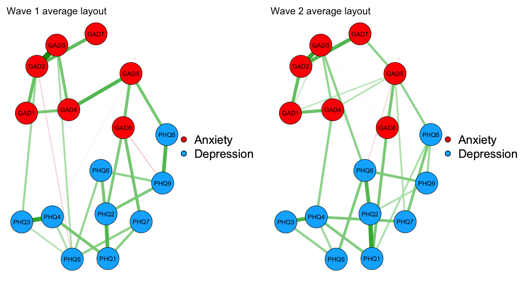
layout(t(1:2))
maxIsing2<-max(c(network1_mod2_graph, network2_mod2_graph))
network1_mod2_plot_average <- qgraph(network1_mod2_graph,
                                     layout=L,
                                     title="Wave 1 average layout",
                                     labels=labels_time1and2data,
                                     groups = groups_time1and2data,
                                     maximum=maxIsing2)
network2_mod2_plot_average <- qgraph(network2_mod2_graph,
                                     layout=L,
                                     title="Wave 2 average layout",
                                     labels=labels_time1and2data,
                                     groups = groups_time1and2data,
                                     maximum=maxIsing2)
```
:::
## Results
### Correlations of Network Characteristics Across Waves
To assess test-retest reliability, we correlate edge weights and node strength centrality between Wave 1 and Wave 2 for each estimation model.
::: panel-tabset
#### Model 1: EBICglasso
```{r}
#| code-summary: "Edge weight and centrality correlations across waves (Model 1)"
library(tidyverse)
library(gt)

# Edge weight correlation (upper triangle only, all edges including zeros)
edges1 <- network1$graph[upper.tri(network1$graph)]
edges2 <- network2$graph[upper.tri(network2$graph)]

# Nonzero edges in either wave
nonzero_mask <- edges1 != 0 | edges2 != 0

cor_edges_all    <- cor(edges1, edges2)
cor_edges_nonzero <- cor(edges1[nonzero_mask], edges2[nonzero_mask])

# Node strength centrality correlation
str1 <- centrality(network1$graph)$OutDegree
str2 <- centrality(network2$graph)$OutDegree
cor_strength <- cor(str1, str2)

# Summary table
tibble(
  Measure = c(
    "Edge weights (all pairs)",
    "Edge weights (non-zero in either wave)",
    "Node strength centrality"
  ),
  `Wave 1 – Wave 2 correlation` = round(c(cor_edges_all, cor_edges_nonzero, cor_strength), 3)
) |>
  gt() |>
  tab_header(title = "Test-retest reliability: Model 1 (EBICglasso)") |>
  cols_align(align = "center", columns = 2)
```
```{r}
#| code-summary: "Scatter plot of edge weights across waves (Model 1)"
#| fig-width: 5
#| fig-height: 5
tibble(Wave1 = edges1, Wave2 = edges2) |>
  ggplot(aes(Wave1, Wave2)) +
  geom_point(alpha = 0.5, color = "#4682B4") +
  geom_smooth(method = "lm", se = TRUE, color = "#B4464B") +
  annotate("text", x = Inf, y = -Inf, hjust = 1.1, vjust = -0.5,
           label = paste0("r = ", round(cor_edges_all, 3))) +
  labs(title = "Edge weights: Wave 1 vs Wave 2 (Model 1)",
       x = "Wave 1 edge weight", y = "Wave 2 edge weight") +
  theme_minimal()
```
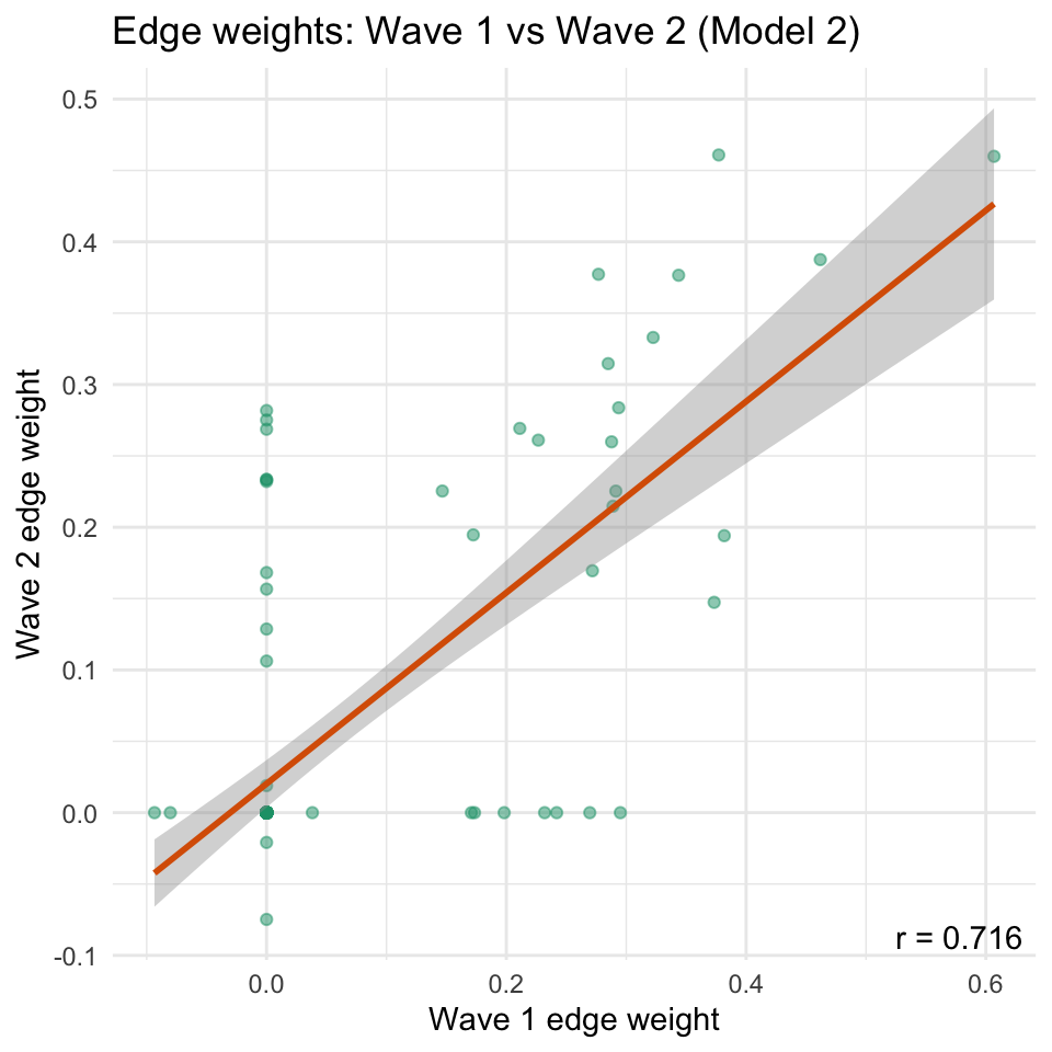
#### Model 2: FIML + Prune
```{r}
#| code-summary: "Edge weight and centrality correlations across waves (Model 2)"
edges1_m2 <- network1_mod2_graph[upper.tri(network1_mod2_graph)]
edges2_m2 <- network2_mod2_graph[upper.tri(network2_mod2_graph)]

nonzero_mask_m2 <- edges1_m2 != 0 | edges2_m2 != 0

cor_edges_all_m2     <- cor(edges1_m2, edges2_m2)
cor_edges_nonzero_m2 <- cor(edges1_m2[nonzero_mask_m2], edges2_m2[nonzero_mask_m2])

str1_m2 <- centrality(network1_mod2_graph)$OutDegree
str2_m2 <- centrality(network2_mod2_graph)$OutDegree
cor_strength_m2 <- cor(str1_m2, str2_m2)

tibble(
  Measure = c(
    "Edge weights (all pairs)",
    "Edge weights (non-zero in either wave)",
    "Node strength centrality"
  ),
  `Wave 1 – Wave 2 correlation` = round(c(cor_edges_all_m2, cor_edges_nonzero_m2, cor_strength_m2), 3)
) |>
  gt() |>
  tab_header(title = "Test-retest reliability: Model 2 (FIML + Prune)") |>
  cols_align(align = "center", columns = 2)
```
```{r}
#| code-summary: "Scatter plot of edge weights across waves (Model 2)"
#| fig-width: 5
#| fig-height: 5
tibble(Wave1 = edges1_m2, Wave2 = edges2_m2) |>
  ggplot(aes(Wave1, Wave2)) +
  geom_point(alpha = 0.5, color = "#1B9E77") +
  geom_smooth(method = "lm", se = TRUE, color = "#D95F02") +
  annotate("text", x = Inf, y = -Inf, hjust = 1.1, vjust = -0.5,
           label = paste0("r = ", round(cor_edges_all_m2, 3))) +
  labs(title = "Edge weights: Wave 1 vs Wave 2 (Model 2)",
       x = "Wave 1 edge weight", y = "Wave 2 edge weight") +
  theme_minimal()
```
:::
## Discussion
### Reliability Estimates Are Method-Dependent
A striking pattern in the results is that the two estimation approaches yield markedly different cross-wave correlations of edge weights.
The EBICglasso solution (Model 1) tends to produce higher test-retest correlations than the FIML-with-pruning solution (Model 2).
This divergence is not incidental — it reflects a fundamental property of regularized versus likelihood-based estimation.
EBICglasso applies $\ell_1$ penalization, which shrinks small edges to exactly zero and retains only the most stable, high-magnitude edges.
Because many small, noisy edges are suppressed in both waves, the surviving edges are structurally more consistent, inflating the apparent reliability.
FIML with pruning, by contrast, retains edges based on a significance threshold without imposing the same magnitude-driven shrinkage, so more variable small edges remain in the estimated graph.
The implication is uncomfortable: **reliability estimates in network psychometrics are not a pure property of the construct being measured — they are partly a property of the estimation algorithm.**
A researcher who chooses EBICglasso may conclude the network is highly replicable; a researcher who chooses FIML may reach a far more skeptical conclusion from the same data.
This method-dependence cautions against interpreting any single reliability index as a definitive verdict on the stability of a psychological network, and underscores the value of multi-model comparisons such as the one conducted here [@forbesQuantifyingReliabilityReplicability2021].
### High Centrality Reliability Does Not Imply Symptom Stability
Even when node strength centrality correlates highly across waves — indicating that the *rank order* of node importance is preserved — this does not license the conclusion that group-level symptom severity is stable.
Centrality reliability is a statement about the *relative* configuration of the network: node $A$ is more central than node $B$ at both time points.
It says nothing about whether the *absolute* level of symptoms has changed, whether the network has become more or less densely connected overall, or whether the clinical burden of any particular symptom has shifted.
Consider a scenario where all symptoms improve substantially between waves (e.g., due to natural recovery or regression to the mean), but the rank order of centrality is preserved.
The centrality correlation would be high, yet the group's symptom profile has changed meaningfully.
Conversely, a population under increasing stress might show rising symptom levels with a reshuffled centrality structure, yielding low reliability despite a clinically important signal.
This distinction matters for practice.
If clinicians or researchers use centrality to identify *treatment targets* — the "most important" nodes to intervene on — high reliability reassures them that the target is a consistent structural feature of the network.
But it provides no guarantee that successfully reducing that symptom will produce the same downstream effects at a later time point, because the network's overall activation level and edge magnitudes may have shifted substantially.
Reliability of rank order and stability of group-level psychopathology are orthogonal quantities, and conflating them risks overstating the clinical utility of network-based intervention targets.