moments::skewness(c(1:10, 100))[1] 2.793716moments::skewness(rnorm(100, 0, 1))[1] 0.1482851moments::skewness(c(1:10, 100))[1] 2.793716moments::skewness(rnorm(100, 0, 1))[1] 0.1482851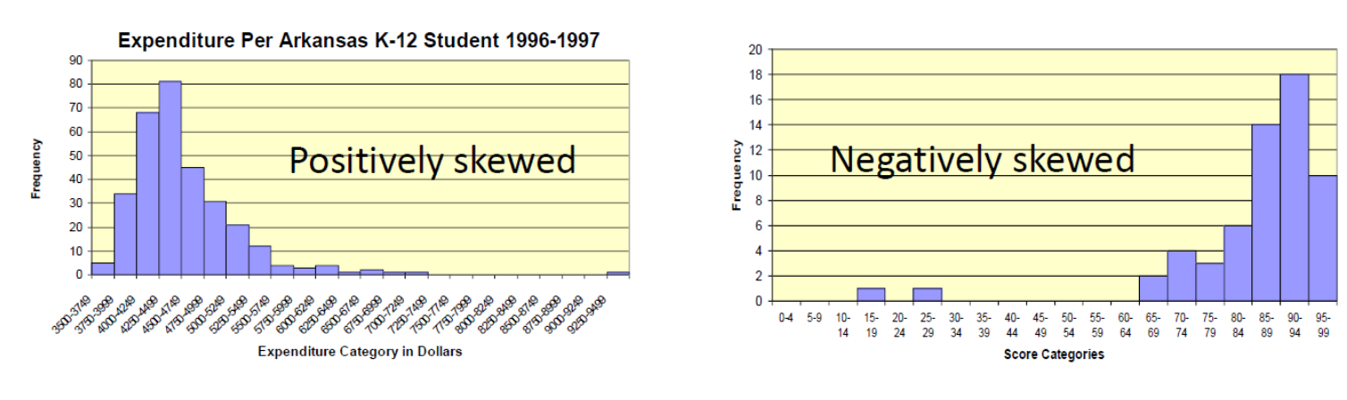
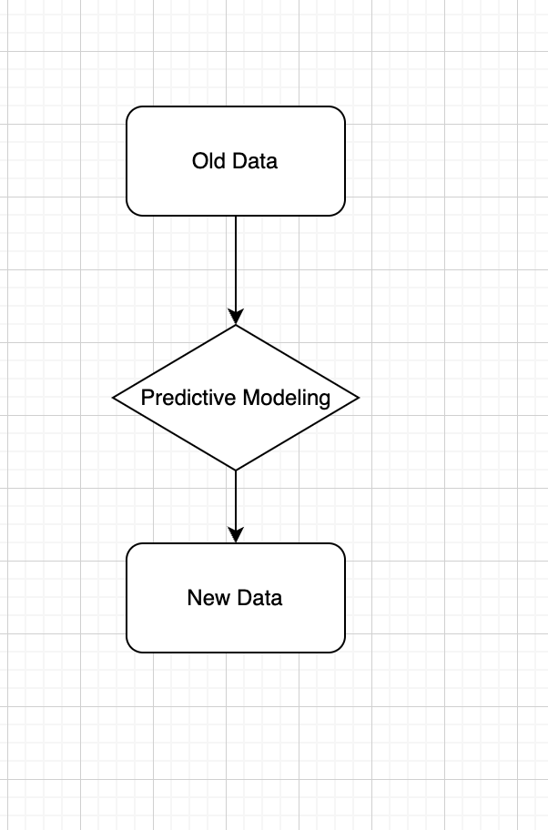
Definition: Use observed data to produce the most accurate prediction possible for new data. Here, the primary goal is that the predicted values have the highest possible fidelity to the true value of the new data.
Example: A simple example would be for a book buyer to predict how many copies of a particular book should be shipped to their store for the next month.
How many houses burned in California wildfire in the first week?
Which factor is most important causing the fires?
How likely the California wildfire will not happen again in next 5 years?
How likely human will live on Mars?
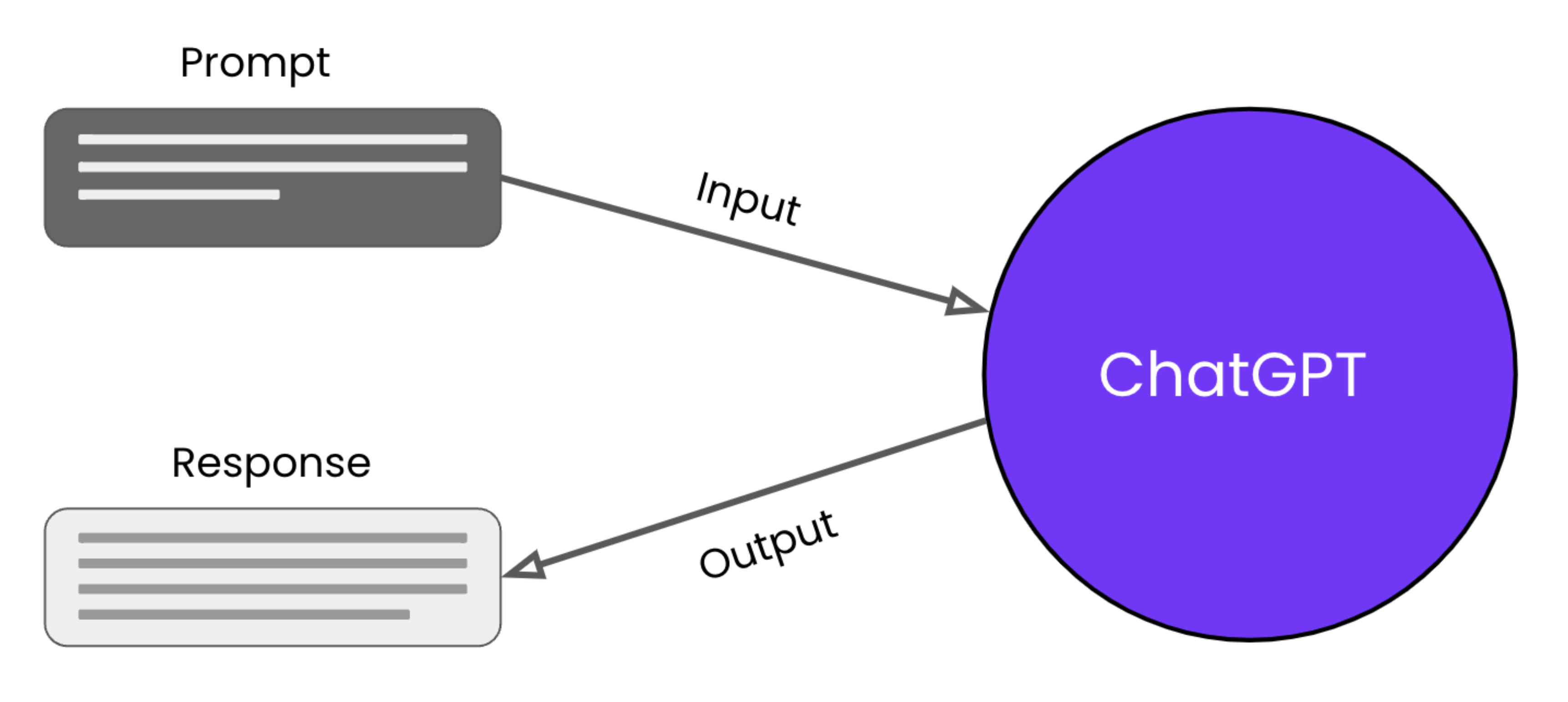
Which type of statistics used by ChatGPT?
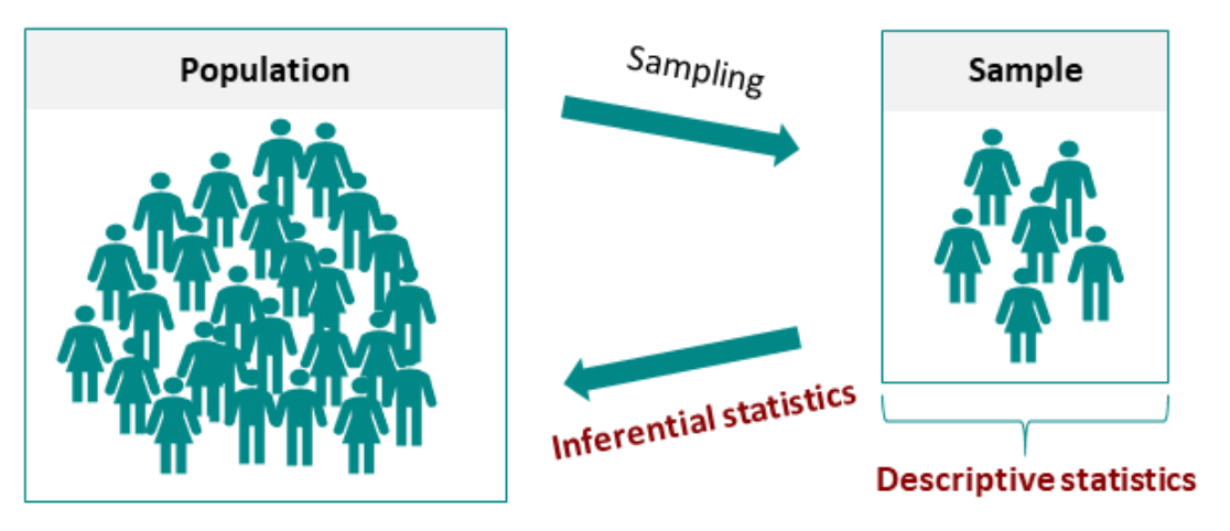
To perform inference statistics, we need to go through following steps:
One-Way ANOVA
Purpose: Tests one factor with three or more levels on a continuous outcome.
Use Case: Comparing means across multiple groups (e.g., diet types on weight loss).
Two-Way ANOVA
Purpose: Examines two factors and their interaction on a continuous outcome.
Use Case: Studying effects of diet and exercise on weight loss.
Repeated Measures ANOVA
Purpose: Tests the same subjects under different conditions or time points.
Use Case: Longitudinal studies measuring the same outcome over time (e.g., cognitive tests after varying sleep durations).
Mixed-Design ANOVA
Purpose: Combines between-subjects and within-subjects factors in one analysis.
Use Case: Evaluating treatment effects over time with control and experimental groups.
Multivariate Analysis of Variance (MANOVA)
Purpose: Assesses multiple continuous outcomes (dependent variables) influenced by independent variables.
Use Case: Impact of psychological interventions on anxiety, stress, and self-esteem.
party: Democrats (4), Republicans (5), Independents (8)scores: attitudes scores for the survey respondents
remotes::install_github("JihongZ/ESRM64103")
library(ESRM64103)library(ESRM64103)
library(dplyr)
exp_political_attitude party scores
1 Democrat 4
2 Democrat 3
3 Democrat 5
4 Democrat 4
5 Democrat 4
6 Republican 6
7 Republican 5
8 Republican 3
9 Republican 7
10 Republican 4
11 Republican 5
12 Independent 8
13 Independent 9
14 Independent 8
15 Independent 7
16 Independent 8Standard deviations and variances for each group
Grand mean: 5.625
# Grand mean
mean(exp_political_attitude$scores)
[1] 5.625exp_political_attitude$party <- factor(exp_political_attitude$party, levels = c("Democrat", "Republican", "Independent"))
mean_byGroup <- exp_political_attitude |>
group_by(party) |>
summarise(Mean = mean(scores),
SD = round(sd(scores), 2),
Vars = round(var(scores), 2),
N = n())
mean_byGroup# A tibble: 3 × 5
party Mean SD Vars N
<fct> <dbl> <dbl> <dbl> <int>
1 Democrat 4 0.71 0.5 5
2 Republican 5 1.41 2 6
3 Independent 8 0.71 0.5 5library(ggplot2)
ggplot(data = mean_byGroup) +
geom_bar(mapping = aes(x = party, y = Mean, fill = party), stat = "identity", width = .5) +
geom_label(aes(x = party, y = Mean, label = Mean), nudge_y = .3) +
labs(title = "Attitudes Toward the Tax Return") +
theme(text = element_text(size = 15))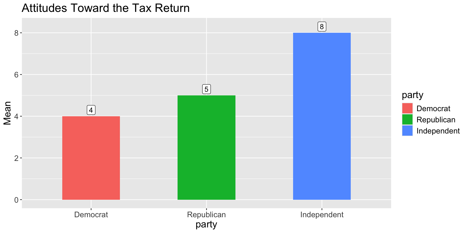
State the null hypothesis and alternative hypothesis:
Set the significant alpha = 0.05
Quick Review of F-statistics:
GrandMean <- mean(exp_political_attitude$scores)
## Between-group Sum of Squares
sum(mean_byGroup$N * (mean_byGroup$Mean - GrandMean)^2)
## Within-group Sum of Squares
SSw_dt <- exp_political_attitude |>
  group_by(party) |>
  mutate(GroupMean = mean(scores),
         Diff_sq = (scores - GroupMean)^2)
sum(SSw_dt$Diff_sq)mod1 <- lm(scores ~ party, data = exp_political_attitude)
anova(mod1)Analysis of Variance Table
Response: scores
Df Sum Sq Mean Sq F value Pr(>F)
party 2 43.75 21.8750 20.312 9.994e-05 ***
Residuals 13 14.00 1.0769
---
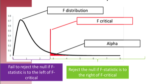
Signif. codes: 0 '***' 0.001 '**' 0.01 '*' 0.05 '.' 0.1 ' ' 1Results show rejection of H₀ (F_obs > F_critical)
F-statistic has two degree of freedoms. This is the density distribution of F-statistics for degree of freedoms as 2 and 13.
# Set degrees of freedom for the numerator and denominator
num_df <- 2  # Change this as per your specification
den_df <- 13  # Change this as per your specification

# Generate a sequence of F values
f_values <- seq(0, 8, length.out = 1000)

# Calculate the density of the F-distribution
f_density <- df(f_values, df1 = num_df, df2 = den_df)

# Create a data frame for plotting
data_to_plot <- data.frame(F_Values = f_values, Density = f_density)
data_to_plot$Reject05 <- data_to_plot$F_Values > 3.81
data_to_plot$Reject01 <- data_to_plot$F_Values > 6.70
# Plot the density using ggplot2
ggplot(data_to_plot) +
  geom_area(aes(x = F_Values, y = Density), fill = "grey",
            data = filter(data_to_plot, !Reject05)) + # Draw the line
  geom_area(aes(x = F_Values, y = Density), fill = "yellow",
            data = filter(data_to_plot, Reject05)) + # Draw the line
  geom_area(aes(x = F_Values, y = Density), fill = "tomato",
            data = filter(data_to_plot, Reject01)) + # Draw the line
  geom_vline(xintercept = 3.81, linetype = "dashed", color = "red") +
  geom_label(label = "F_crit = 3.81 (alpha = .05)", x = 3.81, y = .5, color = "red") +
  geom_vline(xintercept = 6.70, linetype = "dashed", color = "royalblue") +
  geom_label(label = "F_crit = 6.70 (alpha = .01)", x = 6.70, y = .5, color = "royalblue") +
  ggtitle("Density of F-Distribution") +
  xlab("F values") +
  ylab("Density") +
  theme_classic()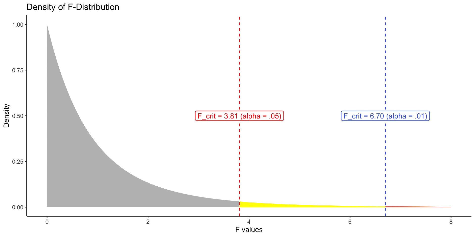
Set the alpha (i.e., type I error rate)—rejection rate, vs. p-value
Alpha can determine several values for the statistical hypothesis testing: the critical value of the test statistics, the rejection region, etc.
Large sample size needs lower alpha level : .01/.001 (more restrict rejection rate)
When we conduct a hypothesis testing, these four cases might be occured
| Reality | ||
| Decision | True | False |
| Fail to reject | Correct Decision | Error made. Type II error (). |
| Reject | Error made. Type I error () |
Correct Decision (Power) |
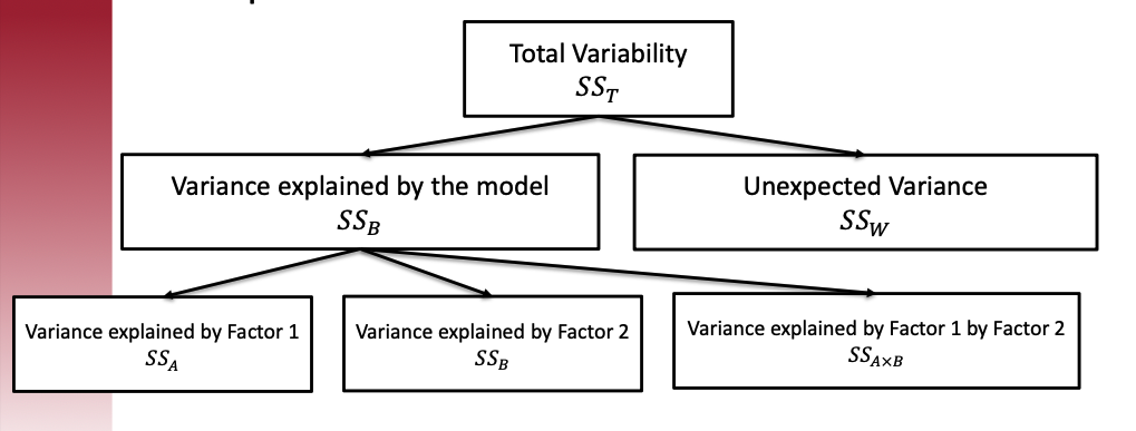
Investigate where the variability of outcome come from?
In this study, do people’s attitude scores differ because of political parties?
Imagine we have two factors: A and B, the variability of outcome can be separated as following:
Core idea of F-stats: comparing the variances between groups and within groups to ascertain if the means of different groups are significantly different from each other.
Logic: if the between-group variance (due to systematic differences caused by the independent variable) is significantly greater than the within-group variance (attributable to random error), the observed differences between group means are likely not due to chance.
F-statistics under 1-way ANOVA:
A one-way ANOVA was conducted to compare the level of concern for tax reform among three political groups: Democrats, Republicans, and Independents. There was a significant effect of political affiliation on tax reform concern at the p < .001 level for the three conditions [F(2, 13) = 20.31, p < .001]. This result indicates significant differences in the attitudes toward tax reform among the groups.
Relying solely on p-values to reject the null hypothesis can be problematic for several reasons:
Binary Decision Making: The use of a threshold (e.g., α = 0.05) to determine whether to reject the null hypothesis reduces the complexity of the data and the underlying phenomena to a binary decision. This can oversimplify the interpretation and overlook the nuances in the data.
Neglect of Effect Size: P-values do not convey the size or importance of an effect. A very small effect can produce a small p-value if the sample size is large enough, leading to a rejection of the null hypothesis even when the effect may not be practically significant.
Probability of Extremes Under the Null: Since p-values quantify the extremeness of the observed data under the null hypothesis, they do not address whether similarly extreme data could also occur under alternative hypotheses. This can lead to an overemphasis on the null hypothesis and potentially disregard other plausible explanations for the data.
A study investigates the effect of different sleep durations on the academic performance of university students. Three groups are defined based on nightly sleep duration: Less than 6 hours, 6 to 8 hours, and more than 8 hours.
We can simulate the data
# Set seed for reproducibility
set.seed(42)

# Generate data for three sleep groups
less_than_6_hours <- rnorm(30, mean = 65, sd = 10)
six_to_eight_hours <- rnorm(50, mean = 75, sd = 8)
more_than_8_hours <- rnorm(20, mean = 78, sd = 7)

# Combine data into a single data frame
sleep_data <- data.frame(
  Sleep_Group = factor(c(rep("<6 hours", 30), rep("6-8 hours", 50), rep(">8 hours", 20))),
  Exam_Score = c(less_than_6_hours, six_to_eight_hours, more_than_8_hours)
)

# View the first few rows of the dataset
head(sleep_data)Groups:
Less than 6 hours: 30 students
6 to 8 hours: 50 students
More than 8 hours: 20 students
Performance Metric: Average exam scores out of 100.
Less than 6 hours: Mean = 65, SD = 10
6 to 8 hours: Mean = 75, SD = 8
More than 8 hours: Mean = 78, SD = 7
Analysis: One-way ANOVA was conducted to compare the average exam scores among the three groups.
Results: F_observed = XX.XX, p = 0.001
Alpha Level: α = 0.05
P-value Interpretation: The p-value (0.001) is less than the alpha level (0.05), indicating a statistically significant difference in exam scores among the different sleep groups.
Conclusion: The results suggest that the amount of sleep significantly affects academic performance, with students getting 6 hours or more of sleep performing better on average than those with less sleep. The findings highlight the importance of adequate sleep among students for optimal academic outcomes.
Due on 02/03 5PM.