1.1 Lecture Outline
- Homework assignment
- Introduction to ANOVA
- Why use ANOVA instead of multiple t-tests?
- Logic and components of ANOVA
- Steps and assumptions in ANOVA
- Example scenario and real-world applications
- Performing ANOVA in R
- Checking homogeneity of variance
- Post-hoc analysis
- Using weights in ANOVA
- Where to find weights for ANOVA
- Conclusion
2 Homework 1
2.1 Let’s walk through HW1
3 One-Way ANOVA
3.1 Introduction
- Overview of ANOVA and its applications.
- Used for comparing means across multiple groups.
- Explanation of why ANOVA is essential in statistical analysis.
3.2 ANOVA Basics
- Analysis of Variance (ANOVA) compares multiple group means (more than two groups).
- If comparing only 2 groups, either a t-test or an F-test can be used.
- When more than 2 groups are compared, an F-test (ANOVA) is required.
3.3 Why Use ANOVA Instead of Multiple t-tests?
- Computational complexity increases with the number of groups.
- Multiple t-tests inflate the Type I error rate.
- ANOVA provides an omnibus test to detect any significant difference.
- Example demonstrating inflated Type I error with multiple t-tests.
3.4 Logic of ANOVA
- ANOVA compares group means by analyzing variance components.
- Two independent variance estimates:
- Between-group variability (treatment effect)
- Within-group variability (error or chance)
- Illustration: Graph showing variance breakdown.
3.5 Components of ANOVA
- Total Sum of Squares (): Total variance of outcomes in the data.
- Sum of Squares Between (): Variability of outcomes due to the group(s).
- Sum of Squares Within (): Variability due to error (some we do not test yet).
- Relationship:
3.5.1 If > …
R output:
            Df Sum Sq Mean Sq F value Pr(>F)
group        1 218.42  218.42   264.1 <2e-16 ***
Residuals   38  31.43    0.83
---
Signif. codes:  0 '***' 0.001 '**' 0.01 '*' 0.05 '.' 0.1 ' ' 1
3.5.2 If < …
R output:
            Df Sum Sq Mean Sq F value Pr(>F)
group        1  113.4  113.43   5.485 0.0245 *
Residuals   38  785.8   20.68
---
Signif. codes:  0 '***' 0.001 '**' 0.01 '*' 0.05 '.' 0.1 ' ' 1
3.6 Practical Steps in One-way ANOVA
- Compute total variability.
- Decompose total variability into model-related and error-related components.
- Compute the F-statistic:
- Construct the ANOVA table, determine alpha level and draw conclusions.
- Examine Homogeneity of Variance
- Conduct Post-Hoc Analysis
3.7 Assumptions of ANOVA
- Independence of observations.
- Normality of residuals.
- Homogeneity of variance (homoscedasticity).
- Consequences of violating these assumptions.
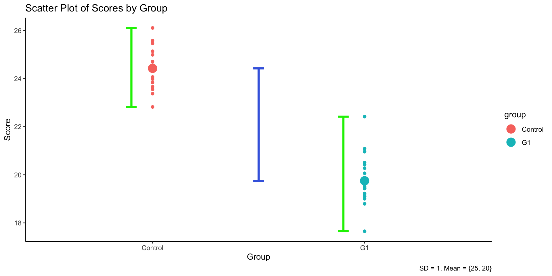
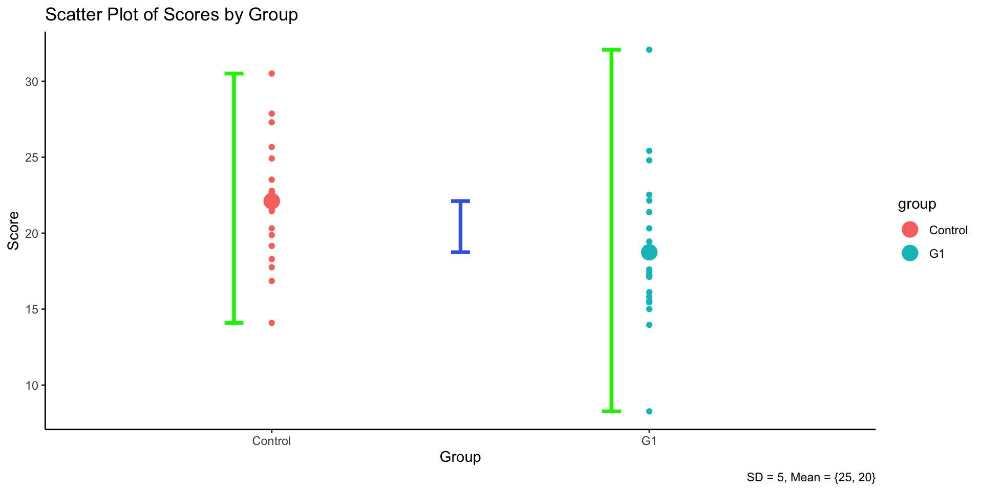
3.8 Homogeneity of Variance
- ANOVA assumes that variance across groups is equal.
- Unequal variances can lead to incorrect conclusions.
- Example illustrating different variance conditions.
We will talk more details about this in the next lecture
3.9 Methods to Check Homogeneity of Variance
- Levene’s Test: Tests for equal variances across groups.
- Bartlett’s Test: Specifically tests for homogeneity in normally distributed data.
- Visual Inspection: Boxplots can help assess variance equality.
- Graph: Example of equal and unequal variance in boxplots.
4 Example: One-way ANOVA in R
4.1 Example Scenario
- Research Aim: Investigating the effect of an teaching intervention on children’s verbal acquisition.
- IV (Factor): Intervention groups (G1, G2, G3, Control).
- DV: Verbal acquisition scores.
- Hypotheses:
- :
- : At least two group means differ.
4.2 Performing ANOVA in R
4.2.1 Load Libraries
library(ggplot2)
library(car) # used for leveneTest; install.packages("car")
4.2.2 Generate Sample Data
rnorm(10, 20, 10) # generate 10 data points from a normal distribution of mean as 20 and SD as 10Context: the example research focus on whether three different teaching methods (labeled as G1, G2, G3) on students’ test scores.
In total, 40 students are assigned to three teaching group and one default teaching group. Each group have 10 samples.
set.seed(1234)
data <- data.frame(
  group = rep(c("G1", "G2", "G3", "Control"), each = 10),
  score = c(rnorm(10, 20, 5), rnorm(10, 25, 5), rnorm(10, 30, 5), rnorm(10, 22, 5))
)
data_unequal <- data.frame(
  group = rep(c("G1", "G2", "G3", "Control"), each = 10),
  score = c(rnorm(10, 20, 10), rnorm(10, 25, 5), rnorm(10, 30, 1), rnorm(10, 22, .1))
)
4.2.3 Conduct ANOVA Test
anova_result <- aov(score ~ group, data = data)
summary(anova_result)
Df Sum Sq Mean Sq F value Pr(>F)
group 3 724.1 241.37 11.45 2.04e-05 ***
Residuals 36 759.2 21.09
---
Signif. codes: 0 '***' 0.001 '**' 0.01 '*' 0.05 '.' 0.1 ' ' 1anova_result2 <- aov(score ~ group, data = data_unequal)
summary(anova_result2) Df Sum Sq Mean Sq F value Pr(>F)
group 3 1413 470.9 19.14 1.37e-07 ***
Residuals 36 886 24.6
---
Signif. codes: 0 '***' 0.001 '**' 0.01 '*' 0.05 '.' 0.1 ' ' 14.3 Checking Homogeneity of Variance
4.3.1 Method 1: Visual Inspection of Variance Equality
Equal Variances across groups
ggplot(data, aes(x = group, y = score)) +
geom_boxplot() +
theme_minimal() +
labs(title = "Boxplot of Scores by Group", x = "Group", y = "Score")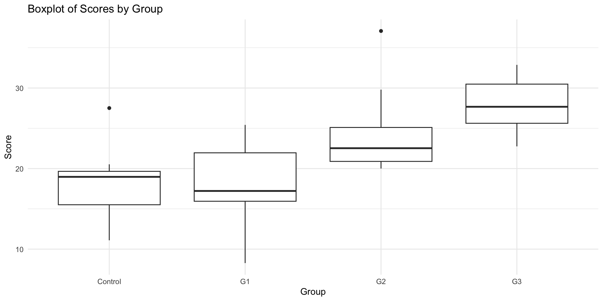
Unequal Variances across groups
ggplot(data_unequal, aes(x = group, y = score)) +
geom_boxplot() +
theme_minimal() +
labs(title = "Boxplot of Scores by Group", x = "Group", y = "Score")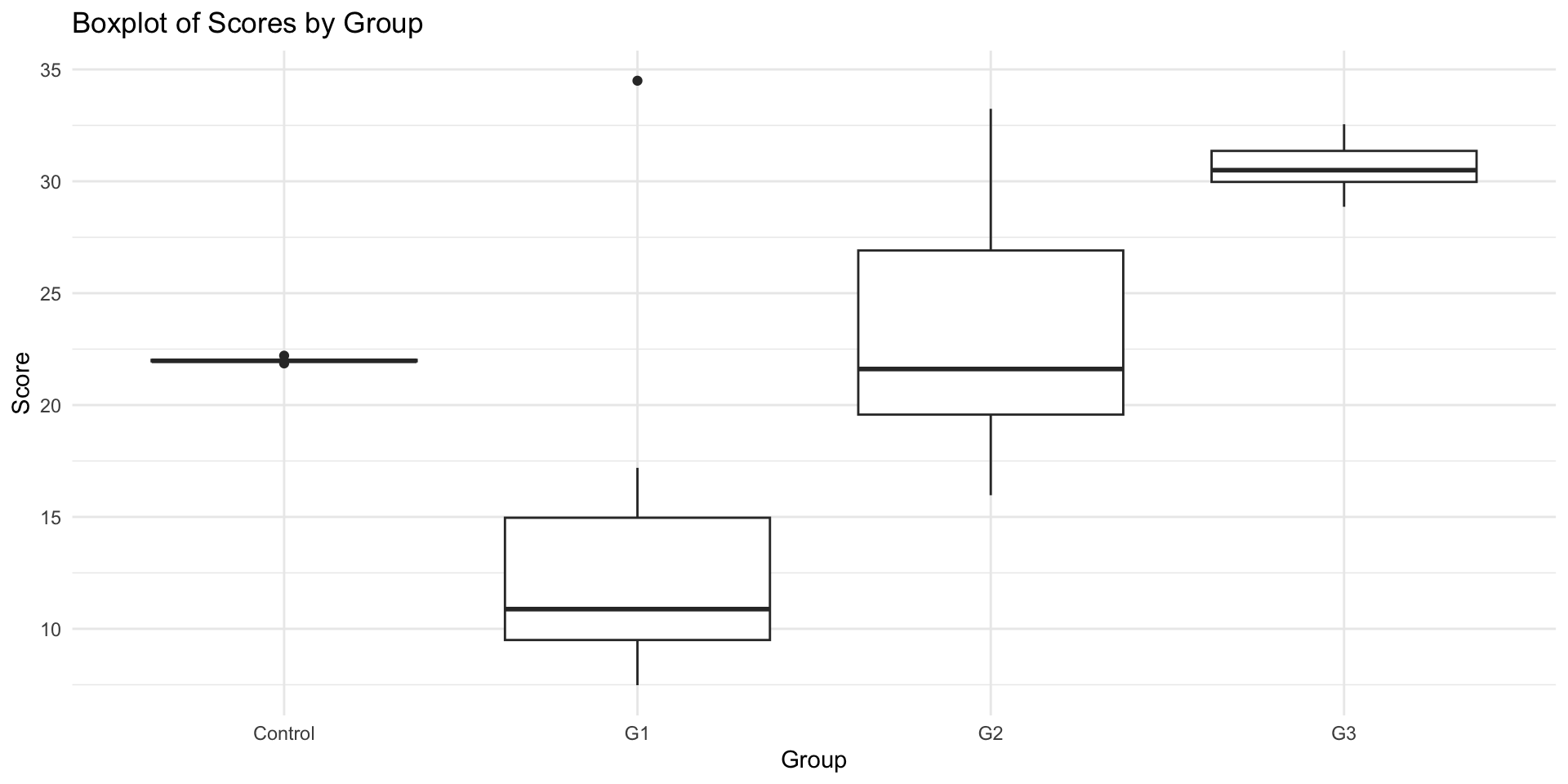
4.3.2 Method 2: Using Bartlett’s Test
bartlett.test(score ~ group, data = data)
Bartlett test of homogeneity of variances
data: score by group
Bartlett's K-squared = 2.0115, df = 3, p-value = 0.57bartlett.test(score ~ group, data = data_unequal)
Bartlett test of homogeneity of variances
data: score by group
Bartlett's K-squared = 82.755, df = 3, p-value < 2.2e-164.3.3 Method 3: Using Levene’s Test
leveneTest(score ~ group, data = data)Levene's Test for Homogeneity of Variance (center = median)
Df F value Pr(>F)
group 3 0.1779 0.9107
36 leveneTest(score ~ group, data = data_unequal)Levene's Test for Homogeneity of Variance (center = median)
Df F value Pr(>F)
group 3 3.4749 0.02581 *
36
---
Signif. codes: 0 '***' 0.001 '**' 0.01 '*' 0.05 '.' 0.1 ' ' 14.4 Post-hoc Analysis
4.4.1 Tukey Honest Significant Differences (HSD) Test
Create a set of confidence intervals on the differences between the means of the pairwise levels of a factor with the specified family-wise probability of coverage.
When comparing the means for the levels of a factor in an analysis of variance, a simple comparison using t-tests will inflate the probability of declaring a significant difference when it is not in fact present.
Based on Tukey’s ‘Honest Significant Differences’ method
tukey_result <- TukeyHSD(anova_result)
print(tukey_result$group) diff lwr upr p adj
G1-Control -0.08482175 -5.6158112 5.446168 0.9999741881
G2-Control 6.24011176 0.7091223 11.771101 0.0218818550
G3-Control 9.89123122 4.3602418 15.422221 0.0001491636
G2-G1 6.32493351 0.7939441 11.855923 0.0197364909
G3-G1 9.97605296 4.4450635 15.507042 0.0001317258
G3-G2 3.65111946 -1.8798700 9.182109 0.3003394077plot(tukey_result)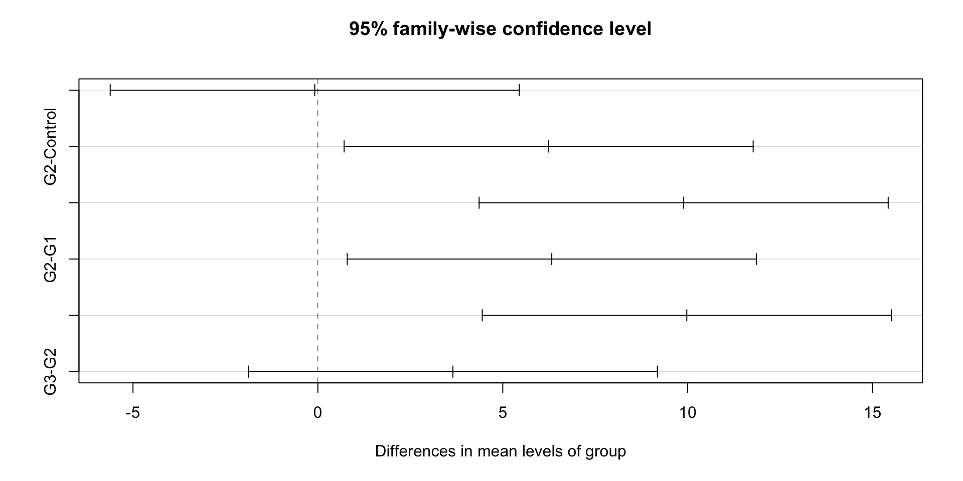
4.5 Interpreting Results
4.5.1 ANOVA Statistics
            Df Sum Sq Mean Sq F value   Pr(>F)
group        3  724.1  241.37   11.45 2.04e-05 ***
Residuals   36  759.2   21.09
---
Signif. codes: 0 '***' 0.001 '**' 0.01 '*' 0.05 '.' 0.1 ' ' 1⌘+C
library(dplyr)
data |>
  group_by(group) |>
  summarise(
    Mean = mean(score),
    SD = sd(score)
  )
# A tibble: 4 × 3
group Mean SD
<chr> <dbl> <dbl>
1 Control 18.2 4.47
2 G1 18.1 4.98
3 G2 24.4 5.34
4 G3 28.1 3.33- A one-way analysis of variance (ANOVA) was conducted to examine the effect of teaching method on students’ test scores. The results indicated a statistically significant difference in test scores across the three teaching methods, ( F(3, 27) = 11.45, p < .001 ). Post-hoc comparisons using the Tukey HSD test revealed that the Interactive method (G3) ( M = 28.06, SD = 3.33 ) resulted in significantly higher scores than the Traditional method ( M = 18.17, SD = 4.47) with the p-value lower than .001, but no significant difference was found between the Interactive (G1) and the traditional methods ( p = .99 ). These results suggest that using interactive teaching methods can improve student performance compared to traditional methods.
4.6 Real-world Applications of ANOVA
- Experimental designs in psychology.
- Clinical trials in medicine.
- Market research and A/B testing.
- Example case studies.
4.7 Using Weights in ANOVA
- In some cases, observations may have different levels of reliability or importance.
- Weighted ANOVA allows us to account for these differences by assigning weights.
- Example: A study where some groups have higher variance and should contribute less to the analysis.
4.8 Example: Applying Weights in aov()
weights <- c(rep(1, 10), rep(2, 10), rep(0.5, 10), rep(1.5, 10))
anova_weighted <- aov(score ~ group, data = data, weights = weights)
summary(anova_weighted)
Df Sum Sq Mean Sq F value Pr(>F)
group 3 666.6 222.20 7.578 0.000471 ***
Residuals 36 1055.5 29.32
---
Signif. codes: 0 '***' 0.001 '**' 0.01 '*' 0.05 '.' 0.1 ' ' 1- The weights modify the influence of each observation in the model.
- Helps in cases where data reliability varies across groups.
4.9 Where Do We Get Weights for ANOVA?
- Weights can be derived from:
- Large-scale assessments: Different student groups may have varying reliability in measurement.
- Survey data: Unequal probability of selection can be adjusted using weights.
- Experimental data: Measurement error models may dictate different weight assignments.
4.10 Example: Using Weights in Large-Scale Assessments
- Consider an educational study where test scores are collected from schools of varying sizes.
- Larger schools may contribute more observations but should not dominate the analysis.
- Weighting adjusts for this imbalance:
weights <- ifelse(data$group == "LargeSchool", 0.5, 1)
anova_weighted <- aov(score ~ group, data = data, weights = weights)
summary(anova_weighted)
Df Sum Sq Mean Sq F value Pr(>F)
group 3 724.1 241.37 11.45 2.04e-05 ***
Residuals 36 759.2 21.09
---
Signif. codes: 0 '***' 0.001 '**' 0.01 '*' 0.05 '.' 0.1 ' ' 1- Ensures fair representation in the analysis.
4.11 Conclusion and Interpretation
- Review results and discuss findings.
- Key takeaways from the analysis.
4.12 Bonus: AI + Statistics
library(ellmer)
chat <- chat_ollama(model = "llama3.2", seed = 1234)

prompt <- paste0("Perform ANOVA analysis using R code given the generated data sets by R and then interpret the results",
'
set.seed(1234)
data <- data.frame(
  group = rep(c("G1", "G2", "G3", "Control"), each = 10),
  score = c(rnorm(10, 20, 5), rnorm(10, 25, 5), rnorm(10, 30, 5), rnorm(10, 22, 5))
)
')
chat$chat(prompt)
Here is an example of how to perform ANOVA analysis using the given data set in
R:
```r
# Load necessary libraries
library(car)
# Perform ANOVA analysis
anova_result <- aov(score ~ group, data = data)
# Print summary of ANOVA results
summary(anova_result)
```
In this code, we first load the necessary "car" library to access the `aov()`
function, which performs the ANOVA analysis. We then perform ANOVA using
`aov()` on our score variable and a categorical independent variable 'group'
and print out the results.
Here is how you can interpret the results:
```
Df Sum Sq Mean Sq F value Pr(>F)
group 3 145.5 48.50 11.41 1.39e-10 ***
Residuals 30 1550.2 51.75
---
Signif. codes: 0 ‘***’ 0.001 ‘**’ 0.01 ‘*’ 0.05 ‘.’ 0.1 ‘ ’ 1
Residual standard error: 7.0556
(multiplied by sqrt())
Number of observations: 40
(All tests are two-tailed)
Multiple R-squared: 0.9635 # near perfect fit
Adjusted R-squared: 0.9517 # a very strong correlation between score and group
F-statistic: 11.412 on 3 and 30 DF, p-value = inf
```
From the results:
- The F-statistic of 11.41, accompanied by an extremely low (almost flat)
p-value of `1.39e-10`, suggests that there is a statistically significant
difference among groups.
- With nearly perfect fit using R-squared value with more than **0.9** the
result supports that prediction model perfectly explains given data and can be
assumed suitable predictor model for other scenarios like forecasting , or
making predictions about scores.
Thus, ANOVA proves that groups are significantly different from one another in
terms of mean scores, supporting the idea that group is a significant predictor
variable in our model.library(ellmer)
chat <- chat_ollama(model = "llama3.2", seed = 1234)
chat$chat("What is the null hypothesis for Bartlett's test?")