#install.packages("lmtest")
library(lmtest)
err1 <- rnorm(100)

## generate regressor and dependent variable
x <- rep(c(-1,1), 50)
y1 <- 1 + x + err1
## perform Durbin-Watson test
dwtest(y1 ~ x)1.1 Class Outline
- Go through three assumptions of ANOVA and their checking statistics
- Post-hoc test for more group comparisons.
- Example: Intervention and Verbal Acquisition
- After-class Exercise: Effect of Sleep Duration on Cognitive Performance
1.2 ANOVA Procedure
- Set hypotheses:
- Null hypothesis (): All group means are equal.
- Alternative hypothesis (): At least one group mean differs.
- Determine statistical parameters:
- Significance level
- Degrees of freedom for between-group () and within-group ()
- Find the critical F-value.
- Compute test statistic:
- Calculate F-ratio based on between-group and within-group variance.
- Compare results:
- Either compare with or -value with .
- If , reject .
1.3 ANOVA Type I Error
- The way to compare the means of multiple groups (i.e., more than two groups)
- Compared to multiple t-tests, the ANOVA does not inflate Type I error rates.
- For F-test in ANOVA, Type I error rate is not inflated
- Type I error rate is inflated when we do multiple comparison
- Family-wise error rate: probability of at least one Type I error occur = where c =number of tests. Frequently used FWER methods include Bonferroni or FDR.
Family-Wise Error Rate
- The Family-Wise Error Rate (FWER) is the probability of making at least one Type I error (false positive) across a set of multiple comparisons.
- In Analysis of Variance (ANOVA), multiple comparisons are often necessary when analyzing the differences between group means. FWER control is crucial to ensure the validity of statistical conclusions.
2 ANOVA Assumptions
2.1 Overview
- Like all statistical tests, ANOVA requires certain assumptions to be met for valid conclusions:
- Independence: Observations are independent of each other.
- Normality: The residuals (errors) follow a normal distribution.
- Homogeneity of variance (HOV): The variance within each group is approximately equal.
2.2 Importance of Assumptions
- If assumptions are violated, the results of ANOVA may not be reliable.
- We call it Robustness as to what degree ANOVAs are not influenced by the violation of assumption.
- Typically:
- ANOVA is robust to minor violations of normality, especially for large sample sizes (Central Limit Theorem).
- Not robust to violations of independence—if independence is violated, ANOVA is inappropriate.
- Moderately robust to HOV violations if sample sizes are equal.
2.3 Assumption 1: Independence
- Definition: Each observation should be independent of others.
- Violations:
- Clustering of data (e.g., repeated measures).
- Participants influencing each other (e.g., classroom discussions).
- Check (Optional): Use the Durbin-Watson test.
- Solution: Repeated Measured ANOVA, Mixed ANOVA, Multilevel Model
- Consequences: If independence is violated, ANOVA results are not valid.
Durbin-Watson (DW) Test
Note
The Durbin-Watson test is primarily used for detecting autocorrelation in time-series data.
In the context of ANOVA with independent groups, residuals are generally assumed to be independent.
- However, it’s still good practice to check this assumption, especially if there’s a reason to suspect potential autocorrelation.
Important
- Properties of DW Statistic:
- : Independence of residual is satisfied.
- Ranges from 0 to 4.
- A value around 2 suggests no autocorrelation.
- Values approaching 0 indicate positive autocorrelation.
- Values toward 4 suggest negative autocorrelation.
- P-value
- P-Value: A small p-value (typically < 0.05) indicates violation of independency
lmtest::dwtest()
Performs the Durbin-Watson test for autocorrelation of disturbances.
The Durbin-Watson test has the null hypothesis that the autocorrelation of the disturbances is 0.
This results suggest there are no autocorrelation at the alpha level of .05.
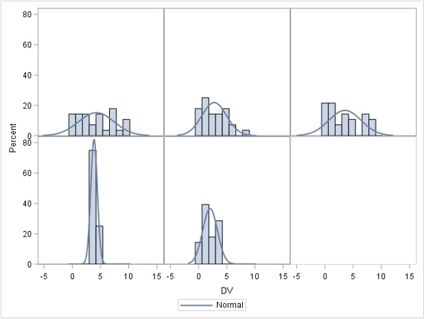
2.4 Assumption 2: Normality
- The dependent variable (DV) should be normally distributed within each group.
- Assessments:
- Graphical methods: Histograms, Q-Q plots.
- Statistical tests:
- Shapiro-Wilk test (common)
- Kolmogorov-Smirnov (KS) test (for large samples)
- Anderson-Darling test (detects kurtosis issues).
- Robustness:
- ANOVA is robust to normality violations for large samples.
- If normality is violated, consider transformations or non-parametric tests.
Normality within Each Group
Assume that the DV (Y) is distributed normally within each group for ANOVA
ANOVA is robust to minor violations of normality
- So generally start with homogeneity, then assess normality
shapiro.test()
set.seed(123)  # For reproducibility
sample_normal_data <- rnorm(200, mean = 50, sd = 10)  # Generate normal data
sample_nonnormal_data <- runif(200, min = 1, max = 10)  # Generate non-normal data

shapiro.test(sample_normal_data)
    Shapiro-Wilk normality test

data:  sample_normal_data
W = 0.99076, p-value = 0.2298shapiro.test(sample_nonnormal_data)
    Shapiro-Wilk normality test

data:  sample_nonnormal_data
W = 0.95114, p-value = 2.435e-06
# Perform Kolmogorov-Smirnov test against a normal distribution
ks.test(scale(sample_normal_data), "pnorm")
    Asymptotic one-sample Kolmogorov-Smirnov test

data:  scale(sample_normal_data)
D = 0.054249, p-value = 0.5983
alternative hypothesis: two-sidedks.test(scale(sample_nonnormal_data), "pnorm")
    Asymptotic one-sample Kolmogorov-Smirnov test

data:  scale(sample_nonnormal_data)
D = 0.077198, p-value = 0.1843
alternative hypothesis: two-sided
2.5 Assumption 3: Homogeneity of Variance (HOV)
- Variance across groups should be equal.
- Assessments:
- Levene’s test: Tests equality of variances.
- Brown-Forsythe test: More robust to non-normality.
- Bartlett’s test: For data with normality.
- Boxplots: Visual inspection.
- What if violated?
- Welch’s ANOVA (adjusted for variance differences).
- Transforming the dependent variable.
- Using non-parametric tests (e.g., Kruskal-Wallis).
Practical Considerations
## Computes Levene's test for homogeneity of variance across groups.
car::leveneTest(outcome ~ group, data = data)

## Boxplots to visualize the variance by groups
boxplot(outcome ~ group, data = data)

## Brown-Forsythe test
onewaytests::bf.test(outcome ~ group, data = data)

## Bartlett's Test
bartlett.test(outcome ~ group, data = data)- Levene’s test and Brown-Forsythe test are often preferred when data does not meet the assumption of normality, especially for small sample sizes.
- Bartlett’s test is most powerful when the data is normally distributed and when sample sizes are equal across groups. However, it can be less reliable if these assumptions are violated.
Decision Tree
library(ellmer)
chat = ellmer::chat_ollama(model = "llama3.2")
chat$chat("How large can be considered as large sample size in one-way ANOVA")
In one-way ANOVA, there is no specific criterion for what constitutes a "large"
sample size. However, here are some general guidelines:
1. **Power**: A commonly used rule of thumb is to require a power of at least
0.8 to detect significant differences between groups. This corresponds to a
sample size of around 20-30 observations per group.
2. **Effect Size**: The effect size (eta^2) measures the proportion of variance
explained by the effect being tested. For one-way ANOVA, a commonly used
threshold for η^2 is 0.05. With this assumption, a large sample size would be
around 50-75 observations per group.
3. **F-statistic**: Another way to evaluate sample size requirements is to set
an F-statistic threshold (e.g., >4.77 for α = 0.05). This corresponds to
approximately 250-375 observations per group.
In general, a larger sample size will increase the power of the test and reduce
the required effect size, which in turn reduces the likelihood of obtaining
significant results by chance. Here are some rough guidelines for minimum
sample sizes:
* Small effect: 10-20 observations per group (power ~0.8)
* Moderate effect: 25-40 observations per group
* Large effect: 50-75 observations per group
Using these guidelines, here are some examples of large sample sizes per group
in one-way ANOVA:
* ≥60 observations per group for a moderate to large effect size (e.g., η^2 =
0.05)
* ≥100 observations per group for a medium-sized effect size
* ≥200 or more observations per group for a small effect size
Keep in mind that these are rough estimates and actually depend on the specific
design, sample characteristics, and research context.
If you need help calculating power or determining whether your data require the
use of certain assumptions (such as equal variances), consult with your
instructor or statistical consulting resources.2.6 ANOVA Robustness
Robust to:
- Minor normality violations (for large samples).
- Small HOV violations if group sizes are equal.
Not robust to:
- Independence violations—ANOVA is invalid if data points are dependent.
- Severe HOV violations—Type I error rates become unreliable.
The robustness of assumptions is something you should be carefull before/when you perform data collection. They are not something you can do after data collection has been finished.
Robustness to Violations of Normality Assumption
ANOVA assumes that the residuals (errors) are normally distributed within each group.
However, ANOVA is generally robust to violations of normality, particularly when the sample size is large.
Theoretical Justification: This robustness is primarily due to the Central Limit Theorem (CLT), which states that, for sufficiently large sample sizes (typically per group), the sampling distribution of the mean approaches normality, even if the underlying population distribution is non-normal.
This means that, unless the data are heavily skewed or have extreme outliers, ANOVA results remain valid and Type I error rates are not severely inflated.
2.6.1 Robustness to Violations of Homogeneity of Variance
The homogeneity of variance (homoscedasticity) assumption states that all groups should have equal variances. ANOVA can tolerate moderate violations of this assumption, particularly when:
Sample sizes are equal (or nearly equal) across groups – When groups have equal sample sizes, the F-test remains robust to variance heterogeneity because the pooled variance estimate remains balanced.
The degree of variance heterogeneity is not extreme – If the largest group variance is no more than about four times the smallest variance, ANOVA results tend to remain accurate.
2.6.2 ANOVA: Lack of Robustness to Violations of Independence of Errors
The assumption of independence of errors means that observations within and between groups must be uncorrelated. Violations of this assumption severely compromise ANOVA’s validity because:
- Inflated Type I error rates – If errors are correlated (e.g., due to clustering or repeated measures), standard errors are underestimated, leading to an increased likelihood of falsely rejecting the null hypothesis.
- Biased parameter estimates – When observations are not independent, the variance estimates do not accurately reflect the true variability in the data, distorting F-statistics and p-values.
- Common sources of dependency – Examples include nested data (e.g., students within schools), repeated measurements on the same subjects, or time-series data. In such cases, alternatives like mixed-effects models or generalized estimating equations (GEE) should be considered.
3 Omnibus ANOVA Test
3.1 Overview
- What does it test?
- Whether there is at least one significant difference among means.
- Limitation:
- Does not tell which groups are different.
- Solution:
- Conduct post-hoc tests.
3.2 Individual Comparisons of Means
- If ANOVA is significant, follow-up tests identify where differences occur.
- Types:
- Planned comparisons: Defined before data collection.
- Unplanned (post-hoc) comparisons: Conducted after ANOVA.
3.3 Planned vs. Unplanned Comparisons
- Planned:
- Based on theory.
- Can be done even if ANOVA is not significant.
- Unplanned (post-hoc):
- Data-driven.
- Only performed if ANOVA is significant.
3.4 Types of Unplanned Comparisons
- Common post-hoc tests:
- Fisher’s LSD
- Bonferroni correction or Adjusted p-values
- Sidák correction
- Tukey’s HSD
Fisher’s LSD
- Least Significant Difference test.
- Problem: Does not control for multiple comparisons (inflated Type I error).
Bonferroni Correction
- Adjusts alpha to reduce Type I error.
- New alpha: (where is the number of comparisons).
- Conservative: Less power, avoids false positives.
Family-wise Error Rate (adjusted p-values)
- Adjusts p-values to reduce Type I error
- Report adjusted p-values (typically larger that original p-values)
Tukey’s HSD
- Controls for Type I error across multiple comparisons.
- Uses a q-statistic from a Tukey table.
- Preferred when all pairs need comparison.
3.5 ANOVA Example: Intervention and Verbal Acquisition
3.5.1 Background
- Research Question: Does an intensive intervention improve students’ verbal acquisition scores?
- Study Design:
- 4 groups: Control, G1, G2, G3 (treatment levels).
- Outcome variable: Verbal acquisition score (average of three assessments).
- Hypotheses:
- : No difference in verbal acquisition scores across groups.
- : At least one group has a significantly different mean.
3.6 Step 1: Generate Simulated Data in R
# Load necessary libraries
library(tidyverse)

# Set seed for reproducibility
set.seed(123)

# Generate synthetic data for 4 groups
data <- tibble(
  group = rep(c("Control", "G1", "G2", "G3"), each = 30),
  verbal_score = c(
    rnorm(30, mean = 70, sd = 10),  # Control group
    rnorm(30, mean = 75, sd = 12),  # G1
    rnorm(30, mean = 80, sd = 10),  # G2
    rnorm(30, mean = 85, sd = 8)    # G3
  )
)

# View first few rows
head(data)
# A tibble: 6 × 2
group verbal_score
<chr> <dbl>
1 Control 64.4
2 Control 67.7
3 Control 85.6
4 Control 70.7
5 Control 71.3
6 Control 87.23.7 Step 2: Summary Statistics
# Summary statistics by group
data %>%
  group_by(group) %>%
  summarise(
    mean_score = mean(verbal_score),
    sd_score = sd(verbal_score),
    n = n()
  )
# A tibble: 4 × 4
group mean_score sd_score n
<chr> <dbl> <dbl> <int>
1 Control 69.5 9.81 30
2 G1 77.1 10.0 30
3 G2 80.2 8.70 30
4 G3 84.2 7.25 30# Boxplot visualization
ggplot(data, aes(x = group, y = verbal_score, fill = group)) +
geom_boxplot() +
theme_minimal() +
labs(title = "Verbal Acquisition Scores Across Groups", y = "Score", x = "Group")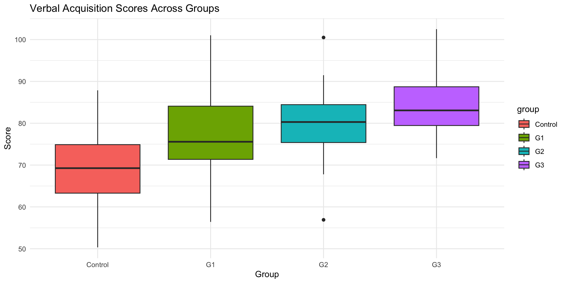
3.8 Step 3: Check ANOVA Assumptions
3.8.1 Assumption Check 1: Independence of residuals Check
# Fit the ANOVA model
anova_model <- lm(verbal_score ~ group, data = data)

# Install lmtest package if not already installed
# install.packages("lmtest")

# Load the lmtest package
library(lmtest)

# Perform the Durbin-Watson test
dw_test_result <- dwtest(anova_model)

# View the test results
print(dw_test_result)
    Durbin-Watson test

data:  anova_model
DW = 2.0519, p-value = 0.5042
alternative hypothesis: true autocorrelation is greater than 0- Interpretation:
- In this example, the
DWvalue is close to 2, and the p-value is greater than 0.05, indicating no significant autocorrelation in the residuals.
- In this example, the
3.8.2 Assumption Check 2: Normality Check
# Shapiro-Wilk normality test for each group
data %>%
  group_by(group) %>%
  summarise(
    shapiro_p = shapiro.test(verbal_score)$p.value
  )
# A tibble: 4 × 2
group shapiro_p
<chr> <dbl>
1 Control 0.797
2 G1 0.961
3 G2 0.848
4 G3 0.568- Interpretation:
- If , normality assumption is not violated.
- If , data deviates from normal distribution.
- Since the data meets the normality requirement and no outliers, we can use Bartlett’s or Levene’s tests for HOV checking.
- Alternative Check: Q-Q Plot
ggplot(data, aes(sample = verbal_score)) +
  geom_qq() + geom_qq_line() +
  facet_wrap(~group) +
  theme_minimal() +
  labs(title = "Q-Q Plot for Normality Check")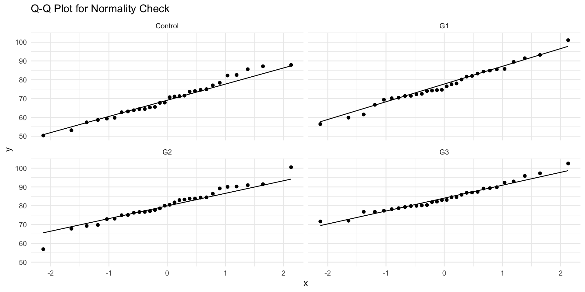
3.8.3 Assumption Check 3: Homogeneity of Variance (HOV) Check
# Levene's Test for homogeneity of variance
car::leveneTest(verbal_score ~ group, data = data)
Levene's Test for Homogeneity of Variance (center = median)
Df F value Pr(>F)
group 3 1.1718 0.3236
116 stats::bartlett.test(verbal_score ~ group, data = data)
    Bartlett test of homogeneity of variances

data:  verbal_score by group
Bartlett's K-squared = 3.5385, df = 3, p-value = 0.3158onewaytests::bf.test(verbal_score ~ group, data = data)
  Brown-Forsythe Test (alpha = 0.05)
-------------------------------------------------------------
  data : verbal_score and group

  statistic  : 14.32875
  num df     : 3
  denom df   : 109.9888
  p.value    : 6.030497e-08

  Result     : Difference is statistically significant.
------------------------------------------------------------- - Interpretation:
- If , variance is homogeneous (ANOVA assumption met).
- If , variance differs across groups (consider Welch’s ANOVA).
- It turns out our data does not violate the homogeneity of variance assumption.
3.9 Step 4: Perform One-Way ANOVA
anova_model <- aov(verbal_score ~ group, data = data)
summary(anova_model)
Df Sum Sq Mean Sq F value Pr(>F)
group 3 3492 1164.1 14.33 5.28e-08 ***
Residuals 116 9424 81.2
---
Signif. codes: 0 '***' 0.001 '**' 0.01 '*' 0.05 '.' 0.1 ' ' 1- Interpretation:
- If , at least one group mean is significantly different.
- If , fail to reject (no significant differences).
3.10 Step 5: Post-Hoc Tests (Tukey’s HSD)
# Tukey HSD post-hoc test
tukey_results <- TukeyHSD(anova_model)
round(tukey_results$group, 3)
diff lwr upr p adj
G1-Control 7.611 1.545 13.677 0.008
G2-Control 10.715 4.649 16.782 0.000
G3-Control 14.720 8.654 20.786 0.000
G2-G1 3.104 -2.962 9.170 0.543
G3-G1 7.109 1.042 13.175 0.015
G3-G2 4.005 -2.062 10.071 0.318- Interpretation:
- Identifies which groups differ.
- If , the groups significantly differ.
- G1-Control
- G2-Control
- G3-Control
- G3-G1
3.10.1 multcomp: Family-wise Error Rate Control
Other multicomparison method allow you to choose which method for adjust p-values.
library(multcomp)
# install.packages("multcomp")
### set up multiple comparisons object for all-pair comparisons
# head(model.matrix(anova_model))
comprs <- rbind(
"G1 - Ctrl" = c(0, 1, 0, 0),
"G2 - Ctrl" = c(0, 0, 1, 0),
"G3 - Ctrl" = c(0, 0, 0, 1),
"G2 - G1" = c(0, -1, 1, 0),
"G3 - G1" = c(0, -1, 0, 1),
"G3 - G2" = c(0, 0, -1, 1)
)
cht <- glht(anova_model, linfct = comprs)
summary(cht, test = adjusted("fdr"))
Simultaneous Tests for General Linear Hypotheses
Fit: aov(formula = verbal_score ~ group, data = data)
Linear Hypotheses:
Estimate Std. Error t value Pr(>|t|)
G1 - Ctrl == 0 7.611 2.327 3.270 0.00283 **
G2 - Ctrl == 0 10.715 2.327 4.604 3.20e-05 ***
G3 - Ctrl == 0 14.720 2.327 6.325 2.94e-08 ***
G2 - G1 == 0 3.104 2.327 1.334 0.18487
G3 - G1 == 0 7.109 2.327 3.055 0.00419 **
G3 - G2 == 0 4.005 2.327 1.721 0.10555
---
Signif. codes: 0 '***' 0.001 '**' 0.01 '*' 0.05 '.' 0.1 ' ' 1
(Adjusted p values reported -- fdr method)3.10.2 Side-by-Side comparison of two methods
TukeyHSD method
             diff    lwr    upr p adj
G1-Control  7.611  1.545 13.677 0.008
G2-Control 10.715  4.649 16.782 0.000
G3-Control 14.720  8.654 20.786 0.000
G2-G1       3.104 -2.962  9.170 0.543
G3-G1       7.109  1.042 13.175 0.015
G3-G2 4.005 -2.062 10.071 0.318FDR method
               Estimate Std. Error t value Pr(>|t|)
G1 - Ctrl == 0    7.611      2.327   3.270  0.00283 **
G2 - Ctrl == 0   10.715      2.327   4.604 3.20e-05 ***
G3 - Ctrl == 0   14.720      2.327   6.325 2.94e-08 ***
G2 - G1 == 0      3.104      2.327   1.334  0.18487
G3 - G1 == 0      7.109      2.327   3.055  0.00419 **
G3 - G2 == 0 4.005 2.327 1.721 0.10555 - The differences in p-value adjustment between the
TukeyHSDmethod and themultcomppackage stem from how each approach calculates and applies the multiple comparisons correction. Below is a detailed explanation of these differences
3.10.3 Comparison of Differences
| Feature | TukeyHSD() (Base R) |
multcomp::glht() |
|---|---|---|
| Distribution Used | Studentized Range (q-distribution) | t-distribution |
| Error Rate Control | Strong FWER control | Flexible error control |
| Simultaneous Confidence Intervals | Yes | Typically not (depends on method used) |
| Adjustment Method | Tukey-Kramer adjustment | Single-step, Westfall, Holm, Bonferroni, etc. |
| P-value Differences | More conservative (larger p-values) | Slightly different due to t-distribution |
3.11 Step 6: Reporting ANOVA Results
Result
We first examined three assumptions of ANOVA for our data as the preliminary analysis. According to the Durbin-Watson test, the Shapiro-Wilk normality test, and the Bartletts’ test, the sample data meets all assumptions of the one-way ANOVA modeling.
A one-way ANOVA was then conducted to examine the effect of three intensive intervention methods (Control, G1, G2, G3) on verbal acquisition scores. There was a statistically significant difference between groups, , .
To further examine which intervention method is most effective, we performed Tukey’s post-hoc comparisons. The results revealed that all three intervention methods have significantly higher scores than the control group (G1-Ctrl: p = .003; G2-Ctrl: p < .001; G3-Ctrl: p < .001). Among three intervention methods, G3 seems to be the most effective. Specifically, G3 showed significantly higher scores than G1 (p = .004). However, no significant difference was found between G2 and G3 (p = .105).
Discussion
These findings suggest that higher intervention intensity improves verbal acquisition performance, which is consistent with prior literatures [xxxx/references]
4 Aftre-Class Exercise: Effect of Sleep Duration on Cognitive Performance
4.1 Background
Research Question:
- Does the amount of sleep affect cognitive performance on a standardized test?
Study Design
- Independent variable: Sleep duration (3 groups: Short (≤5 hrs), Moderate (6-7 hrs), Long (≥8 hrs)).
- Dependent variable: Cognitive performance scores (measured as test scores out of 100).
4.2 Data
# Set seed for reproducibility
set.seed(42)

# Generate synthetic data for sleep study
sleep_data <- tibble(
  sleep_group = rep(c("Short", "Moderate", "Long"), each = 30),
  cognitive_score = c(
    rnorm(30, mean = 65, sd = 10),  # Short sleep group (≤5 hrs)
    rnorm(30, mean = 75, sd = 12),  # Moderate sleep group (6-7 hrs)
    rnorm(30, mean = 80, sd = 8)    # Long sleep group (≥8 hrs)
  )
)

# View first few rows
head(sleep_data)
# A tibble: 6 × 2
sleep_group cognitive_score
<chr> <dbl>
1 Short 78.7
2 Short 59.4
3 Short 68.6
4 Short 71.3
5 Short 69.0
6 Short 63.9Go through all six steps.
4.3 Answer:
# Step 5: Perform One-Way ANOVA
anova_sleep <- aov(cognitive_score ~ sleep_group, data = sleep_data)
summary(anova_sleep)
Df Sum Sq Mean Sq F value Pr(>F)
sleep_group 2 3764 1881.9 15.88 1.32e-06 ***
Residuals 87 10311 118.5
---
Signif. codes: 0 '***' 0.001 '**' 0.01 '*' 0.05 '.' 0.1 ' ' 1A one-way ANOVA was conducted to examine the effect of sleep duration on cognitive performance.
There was a statistically significant difference in cognitive test scores across sleep groups, ,.
Tukey’s post-hoc test revealed that participants in the Long sleep group (M=81.52,SD=6.27) performed significantly better than those in the Short sleep group (M=65.68,SD=12.55), p<.01.
These results suggest that inadequate sleep is associated with lower cognitive performance.