How to use lavaan package to perform Confirmatory Factor Analysis

Manual

lavaan

Author

Jihong Zhang

Published

November 8, 2017

This is one of my homework in Structural Equation Modeling in Fall 2017. Dr. Templin provided a excelent example showing how to perform Confirmatory Factor Analysis (CFA) using Lavaan Package. I elaborated each step as following.

First, load packages needed: If you don’t have the packages installed below, please use install.packages() to install them.

⌘+C

library(tidyverse)
library(lavaan)
#library(semPlot)
library(psych)
library(knitr)
library(kableExtra)

1 Background

1.1 CFA on Attitude towards Inclusive Education Survey (N = 507)

The affective dimension of attitudes subscale includes 6 items on a 6-point likert scale (1 = Strongly Agree, 6 = Strongly Disagree), measuring teachers’ feelings and emotions associated with inclusive education:

I get frustrated when I have difficulty communicating with students with a disability.
I get upset when students with a disability cannot keep up with the day-to-day curriculum in my classroom.
I get irritated when I am unable to understand students with a disability.
I am uncomfortable including students with a disability in a regular classroom with other students without a disability.
I am disconcerted that students with a disability are included in the regular classroom, regardless of the severity of the disability.
I get frustrated when I have to adapt the curriculum to meet the individual needs of all students.

The sample size (N) is 507, which includes 6 males and 501 females. I used one-factor model as first step. All items are loaded on one general factor - affective attitude towards inclusive education. Higher response score means more positive attitude towards inclusive education.

⌘+C

dat <- read.csv("AttitudeForInclusiveEducation.csv")
# head(dat)
dat2 <- dat %>% select(X,Aff.1:Aff.6)
colnames(dat2) <- c("PersonID", paste0("Aff",1:6))

Tip

Note that for such unbalanced data (# of females >> # of males), the interpretation should be cautious. In the Limitation, authors mentioned that the results can not be overgeneralized to the population.

2 Descriptive Statistics

The descriptive statistics for all items are provided below. It appears that item 4 is the least difficult item as it has the highest mean (\mu = 4.189, sd = 1.317); item 5 is the most difficult item as it has lowest mean score (\mu = 3.604, sd = 1.423). All responses for each item range from 1 to 6 (1 = Strongly agree, 6 = Strongly disagree). Thus, all categories are responded. In term of item discrimination, as item 3 has the largest standard deviation (sd = 1.364) and item 6 has the smallest, item 3 has highest discrimination whearas item 6 has lowest in CTT.

	vars	n	mean	sd	median	trimmed	mad	min	max	range	skew	kurtosis	se
PersonID	1	507	254.000	146.503	254	254.000	188.290	1	507	506	0.000	-1.207	6.506
Aff1	2	507	3.765	1.337	4	3.779	1.483	1	6	5	-0.131	-0.927	0.059
Aff2	3	507	3.635	1.335	4	3.636	1.483	1	6	5	-0.026	-0.963	0.059
Aff3	4	507	3.493	1.364	3	3.472	1.483	1	6	5	0.124	-0.969	0.061
Aff4	5	507	4.189	1.317	4	4.287	1.483	1	6	5	-0.589	-0.327	0.058
Aff5	6	507	3.604	1.423	4	3.590	1.483	1	6	5	0.000	-0.939	0.063
Aff6	7	507	4.018	1.313	4	4.061	1.483	1	6	5	-0.356	-0.733	0.058

Item-total correlation table was provided below. All item-total correlation coefficients are higher than 0.7, which suggests good internal consistence. Item 1 has lowest item-total correlation (r = 0.733, sd = 1.337).

Item-total Correlation Table
	n	raw.r	std.r	r.cor	r.drop	mean	sd
Aff1	507	0.733	0.735	0.652	0.611	3.765	1.337
Aff2	507	0.835	0.836	0.806	0.753	3.635	1.335
Aff3	507	0.813	0.812	0.771	0.718	3.493	1.364
Aff4	507	0.789	0.790	0.742	0.689	4.189	1.317
Aff5	507	0.774	0.769	0.702	0.658	3.604	1.423
Aff6	507	0.836	0.838	0.805	0.755	4.018	1.313

2.1 Sample Correlation Matrix

According to Pearson Correlation Matrix below, we can see all items have fairly high pearson correlation coefficients ranging from 0.44 to 0.72. This provides the evidence of dimensionality. Item 2 and item 3 has highest correlation coefficient(r_{23} = 0.717). The lowest correlations lies between item 1 and item 4 as well as item 1 and item 5.

⌘+C

cor(dat2[2:7]) %>% round(3) %>% kable(caption = "Pearson Correlation Matrix")

Pearson Correlation Matrix
	Aff1	Aff2	Aff3	Aff4	Aff5	Aff6
Aff1	1.000	0.590	0.525	0.448	0.411	0.538
Aff2	0.590	1.000	0.717	0.534	0.553	0.602
Aff3	0.525	0.717	1.000	0.505	0.527	0.608
Aff4	0.448	0.534	0.505	1.000	0.609	0.682
Aff5	0.411	0.553	0.527	0.609	1.000	0.577
Aff6	0.538	0.602	0.608	0.682	0.577	1.000

2.2 Sample Mean and Variance

⌘+C

means <- dat2[,2:7] %>% 
  summarise_all(funs(mean)) %>% round(3) %>% t() %>% as.data.frame()
sds <- dat2[,2:7] %>% 
  summarise_all(funs(sd)) %>% round(3) %>% t() %>% as.data.frame()
table1 <- cbind(means,sds)

colnames(table1) <- c("Mean", "SD")
table1

      Mean    SD
Aff1 3.765 1.337
Aff2 3.635 1.335
Aff3 3.493 1.364
Aff4 4.189 1.317
Aff5 3.604 1.423
Aff6 4.018 1.313

2.3 Sample Item Response Distributions

Those items did not exactly match normal distribution but acceptable.

⌘+C

# stack data
dat2_melted <- dat2 %>% gather(key, value,Aff1:Aff6) %>% arrange(PersonID)

# plot by variable
ggplot(dat2_melted, aes(value)) + 
  geom_histogram(aes(y=..density..), colour="black", fill="white", binwidth = 1) +
  geom_density(alpha=.2, fill="#FF6666") +
  scale_x_continuous(breaks = 1:6) +
  facet_wrap(~ key)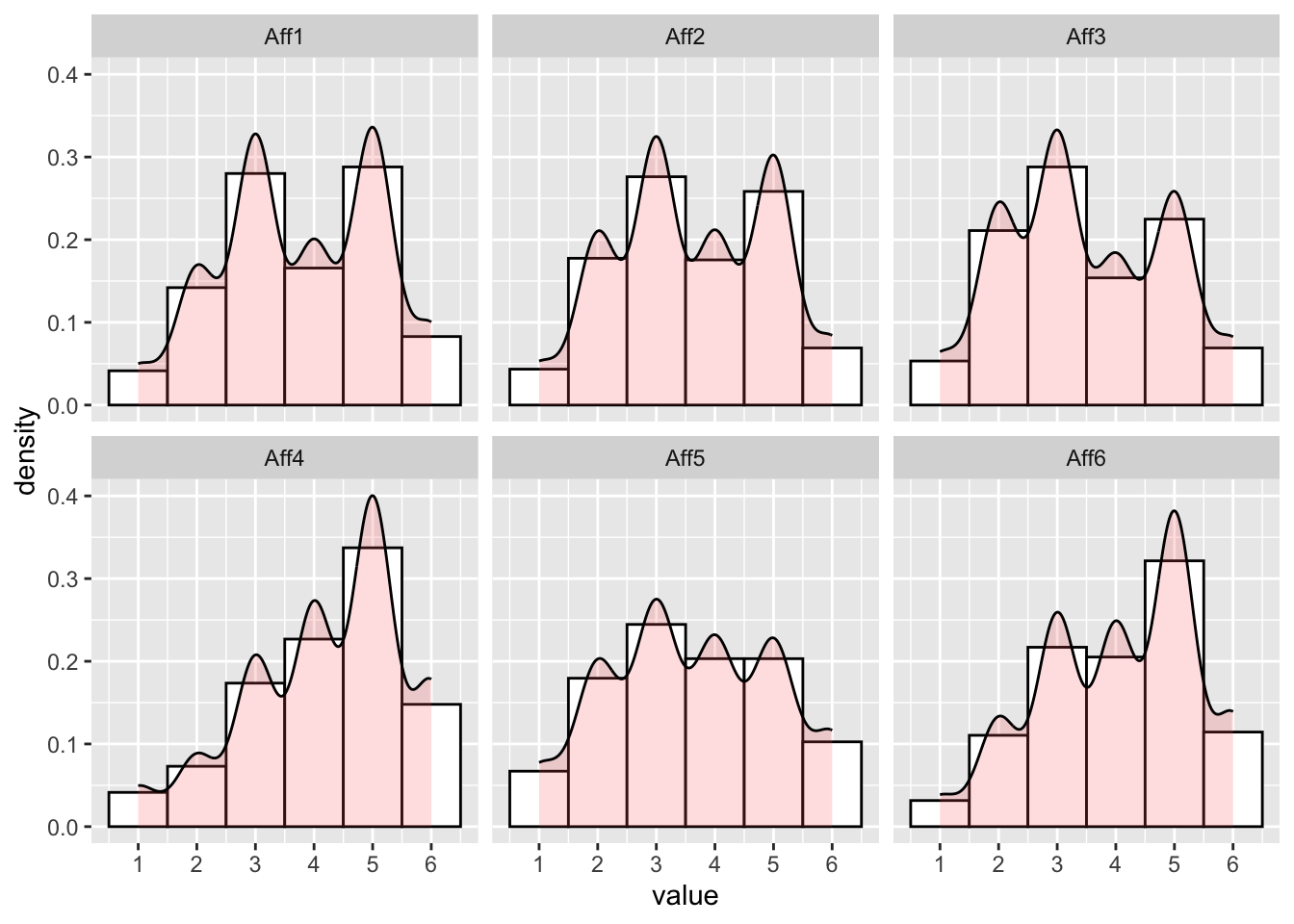

3 Estimation with CFA

3.1 One-factor Model

One-factor model was conducted as first step. The model has one latent facor - affective attitude and six indicators. In general, one-factor model does not provide great model fit except SRMR. The test statistics for chi-square is 75.835 (p < 0.05). CFI is 0.929, which larger than 0.95 suggests good model fit. RMSEA is 0.121, which lower than 0.05 suggest good model fit. SRMR is 0.04, which lower than 0.08. The standardized factor loadings range from 0.66 to 0.8. All factor loadings are significant at the level of alpha equals 0.05.

⌘+C

model1.syntax <- '
  AA =~ Aff1 + Aff2 + Aff3 + Aff4 + Aff5 + Aff6
'
model1 <- cfa(model1.syntax, data = dat2,std.lv = TRUE, mimic = "mplus", estimator = "MLR")
summary(model1, fit.measures = TRUE, standardized = TRUE)

lavaan 0.6.17 ended normally after 14 iterations

  Estimator                                         ML
  Optimization method                           NLMINB
  Number of model parameters                        18

  Number of observations                           507
  Number of missing patterns                         1

Model Test User Model:
                                              Standard      Scaled
  Test Statistic                               115.410      75.834
  Degrees of freedom                                 9           9
  P-value (Chi-square)                           0.000       0.000
  Scaling correction factor                                  1.522
    Yuan-Bentler correction (Mplus variant)                       

Model Test Baseline Model:

  Test statistic                              1573.730     960.267
  Degrees of freedom                                15          15
  P-value                                        0.000       0.000
  Scaling correction factor                                  1.639

User Model versus Baseline Model:

  Comparative Fit Index (CFI)                    0.932       0.929
  Tucker-Lewis Index (TLI)                       0.886       0.882
                                                                  
  Robust Comparative Fit Index (CFI)                         0.934
  Robust Tucker-Lewis Index (TLI)                            0.891

Loglikelihood and Information Criteria:

  Loglikelihood user model (H0)              -4492.146   -4492.146
  Scaling correction factor                                  1.138
      for the MLR correction                                      
  Loglikelihood unrestricted model (H1)      -4434.440   -4434.440
  Scaling correction factor                                  1.266
      for the MLR correction                                      
                                                                  
  Akaike (AIC)                                9020.291    9020.291
  Bayesian (BIC)                              9096.404    9096.404
  Sample-size adjusted Bayesian (SABIC)       9039.270    9039.270

Root Mean Square Error of Approximation:

  RMSEA                                          0.153       0.121
  90 Percent confidence interval - lower         0.129       0.101
  90 Percent confidence interval - upper         0.178       0.142
  P-value H_0: RMSEA <= 0.050                    0.000       0.000
  P-value H_0: RMSEA >= 0.080                    1.000       1.000
                                                                  
  Robust RMSEA                                               0.149
  90 Percent confidence interval - lower                     0.120
  90 Percent confidence interval - upper                     0.181
  P-value H_0: Robust RMSEA <= 0.050                         0.000
  P-value H_0: Robust RMSEA >= 0.080                         1.000

Standardized Root Mean Square Residual:

  SRMR                                           0.040       0.040

Parameter Estimates:

  Standard errors                             Sandwich
  Information bread                           Observed
  Observed information based on                Hessian

Latent Variables:
                   Estimate  Std.Err  z-value  P(>|z|)   Std.lv  Std.all
  AA =~                                                                 
    Aff1              0.886    0.055   16.183    0.000    0.886    0.663
    Aff2              1.078    0.046   23.284    0.000    1.078    0.808
    Aff3              1.066    0.055   19.499    0.000    1.066    0.783
    Aff4              0.968    0.061   15.934    0.000    0.968    0.736
    Aff5              1.004    0.055   18.291    0.000    1.004    0.706
    Aff6              1.057    0.049   21.644    0.000    1.057    0.805

Intercepts:
                   Estimate  Std.Err  z-value  P(>|z|)   Std.lv  Std.all
   .Aff1              3.765    0.059   63.455    0.000    3.765    2.818
   .Aff2              3.635    0.059   61.382    0.000    3.635    2.726
   .Aff3              3.493    0.060   57.741    0.000    3.493    2.564
   .Aff4              4.189    0.058   71.689    0.000    4.189    3.184
   .Aff5              3.604    0.063   57.057    0.000    3.604    2.534
   .Aff6              4.018    0.058   68.948    0.000    4.018    3.062

Variances:
                   Estimate  Std.Err  z-value  P(>|z|)   Std.lv  Std.all
   .Aff1              1.000    0.081   12.285    0.000    1.000    0.560
   .Aff2              0.617    0.066    9.283    0.000    0.617    0.347
   .Aff3              0.719    0.089    8.089    0.000    0.719    0.387
   .Aff4              0.794    0.095    8.390    0.000    0.794    0.459
   .Aff5              1.014    0.090   11.226    0.000    1.014    0.501
   .Aff6              0.605    0.068    8.898    0.000    0.605    0.351
    AA                1.000                               1.000    1.000

3.2 Local Misfit for One-factor Model

By looking into local misfit with residual variance-covariance matrix we can get the clues to improve the model. According to the model residuals, item 4 has relatively high positive residual covariance with item 5 and item 6. It suggests that the one-factor model underestimates the correlations among item 4, item 5 and item 6. In other words, another latent factor may be needed to explain the strong relations among item 4, 5, 6 which cannot be explained by a general Affective attitude factor.

Moreover, modification indices below also suggest that adding the error covariances among item 4, 5 and 6 will improve chi-square much better.

Thus, I decided to add one more factor - AAE. AAE was labeled as affective attitude towards educational environment which indicated by item 4, 5, 6. The other latent factor - AAC which was indicated by item 1, 2, 3 was labeled as Affective Attitude towards communication.

⌘+C

resid(model1)$cov %>% kable(caption = "Normalized Residual Variance-Covariance Matrix",digits = 3)

Normalized Residual Variance-Covariance Matrix
	Aff1	Aff2	Aff3	Aff4	Aff5	Aff6
Aff1	0.000	0.095	0.011	-0.070	-0.109	0.006
Aff2	0.095	0.000	0.153	-0.106	-0.034	-0.085
Aff3	0.011	0.153	0.000	-0.128	-0.051	-0.041
Aff4	-0.070	-0.106	-0.128	0.000	0.168	0.155
Aff5	-0.109	-0.034	-0.051	0.168	0.000	0.015
Aff6	0.006	-0.085	-0.041	0.155	0.015	0.000

⌘+C

modificationindices(model1, standardized = TRUE,sort. = TRUE) %>% slice(1:10) %>% kable(caption = "Modification Indices", digits = 3)

Modification Indices
lhs	op	rhs	mi	epc	sepc.lv	sepc.all	sepc.nox
Aff2	~~	Aff3	55.906	0.319	0.319	0.479	0.479
Aff4	~~	Aff6	45.674	0.279	0.279	0.403	0.403
Aff4	~~	Aff5	25.673	0.243	0.243	0.270	0.270
Aff3	~~	Aff4	24.228	-0.214	-0.214	-0.283	-0.283
Aff2	~~	Aff6	22.494	-0.194	-0.194	-0.318	-0.318
Aff2	~~	Aff4	21.303	-0.193	-0.193	-0.276	-0.276
Aff1	~~	Aff2	11.974	0.153	0.153	0.195	0.195
Aff1	~~	Aff5	7.918	-0.145	-0.145	-0.144	-0.144
Aff1	~~	Aff4	4.309	-0.096	-0.096	-0.108	-0.108
Aff3	~~	Aff6	4.018	-0.084	-0.084	-0.128	-0.128

3.3 Two-factor Model

The neccessity of adding another factor was tested by specifying a two-factor model.

In term of model fit indices, it appears that the global model fit indices are great with two-factor model (CFI = 0.986; RMSEA = 0.058; SRMR = 0.022). Ideally, two latent factors could be labeled as moderately correlated aspects of attitudes towards inclusive education. Thus, the first factor (AAC) could be labeled as how teachers feel about communicating with students with disability. The second (AAE) could be labeled as how teachers feel about evironment of inclusive education. All standardized factor loadings are statistically significant ranging from 0.676 to 0.865. The factor correlation between 2 factors is high (r = 0.838,p = 0.00).

⌘+C

model2.syntax <- '
  AAC =~ Aff1 + Aff2 + Aff3
  AAE =~ Aff4 + Aff5 + Aff6
'
model2 <- cfa(model2.syntax, data = dat2, std.lv = TRUE, mimic = "mplus", estimator = "MLR")
summary(model2, fit.measures = TRUE, standardized = TRUE)

lavaan 0.6.17 ended normally after 19 iterations

  Estimator                                         ML
  Optimization method                           NLMINB
  Number of model parameters                        19

  Number of observations                           507
  Number of missing patterns                         1

Model Test User Model:
                                              Standard      Scaled
  Test Statistic                                32.332      21.512
  Degrees of freedom                                 8           8
  P-value (Chi-square)                           0.000       0.006
  Scaling correction factor                                  1.503
    Yuan-Bentler correction (Mplus variant)                       

Model Test Baseline Model:

  Test statistic                              1573.730     960.267
  Degrees of freedom                                15          15
  P-value                                        0.000       0.000
  Scaling correction factor                                  1.639

User Model versus Baseline Model:

  Comparative Fit Index (CFI)                    0.984       0.986
  Tucker-Lewis Index (TLI)                       0.971       0.973
                                                                  
  Robust Comparative Fit Index (CFI)                         0.987
  Robust Tucker-Lewis Index (TLI)                            0.975

Loglikelihood and Information Criteria:

  Loglikelihood user model (H0)              -4450.606   -4450.606
  Scaling correction factor                                  1.166
      for the MLR correction                                      
  Loglikelihood unrestricted model (H1)      -4434.440   -4434.440
  Scaling correction factor                                  1.266
      for the MLR correction                                      
                                                                  
  Akaike (AIC)                                8939.212    8939.212
  Bayesian (BIC)                              9019.554    9019.554
  Sample-size adjusted Bayesian (SABIC)       8959.246    8959.246

Root Mean Square Error of Approximation:

  RMSEA                                          0.077       0.058
  90 Percent confidence interval - lower         0.051       0.034
  90 Percent confidence interval - upper         0.106       0.082
  P-value H_0: RMSEA <= 0.050                    0.046       0.268
  P-value H_0: RMSEA >= 0.080                    0.475       0.068
                                                                  
  Robust RMSEA                                               0.071
  90 Percent confidence interval - lower                     0.036
  90 Percent confidence interval - upper                     0.108
  P-value H_0: Robust RMSEA <= 0.050                         0.148
  P-value H_0: Robust RMSEA >= 0.080                         0.375

Standardized Root Mean Square Residual:

  SRMR                                           0.022       0.022

Parameter Estimates:

  Standard errors                             Sandwich
  Information bread                           Observed
  Observed information based on                Hessian

Latent Variables:
                   Estimate  Std.Err  z-value  P(>|z|)   Std.lv  Std.all
  AAC =~                                                                
    Aff1              0.903    0.055   16.357    0.000    0.903    0.676
    Aff2              1.153    0.042   27.771    0.000    1.153    0.865
    Aff3              1.117    0.051   22.079    0.000    1.117    0.820
  AAE =~                                                                
    Aff4              1.047    0.053   19.604    0.000    1.047    0.796
    Aff5              1.036    0.053   19.366    0.000    1.036    0.728
    Aff6              1.107    0.044   25.112    0.000    1.107    0.844

Covariances:
                   Estimate  Std.Err  z-value  P(>|z|)   Std.lv  Std.all
  AAC ~~                                                                
    AAE               0.838    0.028   29.829    0.000    0.838    0.838

Intercepts:
                   Estimate  Std.Err  z-value  P(>|z|)   Std.lv  Std.all
   .Aff1              3.765    0.059   63.455    0.000    3.765    2.818
   .Aff2              3.635    0.059   61.382    0.000    3.635    2.726
   .Aff3              3.493    0.060   57.741    0.000    3.493    2.564
   .Aff4              4.189    0.058   71.689    0.000    4.189    3.184
   .Aff5              3.604    0.063   57.057    0.000    3.604    2.534
   .Aff6              4.018    0.058   68.948    0.000    4.018    3.062

Variances:
                   Estimate  Std.Err  z-value  P(>|z|)   Std.lv  Std.all
   .Aff1              0.970    0.083   11.753    0.000    0.970    0.543
   .Aff2              0.449    0.057    7.860    0.000    0.449    0.253
   .Aff3              0.607    0.084    7.244    0.000    0.607    0.327
   .Aff4              0.635    0.085    7.504    0.000    0.635    0.367
   .Aff5              0.950    0.090   10.539    0.000    0.950    0.470
   .Aff6              0.497    0.061    8.191    0.000    0.497    0.288
    AAC               1.000                               1.000    1.000
    AAE               1.000                               1.000    1.000

3.4 Local Misfit for two-factor model

The local misfit indices for two-factor model also suggest that the model fits data well. The largest normalized residuals is 1.215. Modification indices suggest that add covariance between item 5 and item 6. These local misfit is not theoretically defensible. Thus, the final model is two-factor model.

⌘+C

resid(model2)$cov %>% kable(caption = "Normalized Residual Variance-Covariance Matrix",digits = 3)

Normalized Residual Variance-Covariance Matrix
	Aff1	Aff2	Aff3	Aff4	Aff5	Aff6
Aff1	0.000	0.010	-0.053	-0.005	-0.003	0.105
Aff2	0.010	0.000	0.014	-0.075	0.048	-0.016
Aff3	-0.053	0.014	0.000	-0.076	0.050	0.049
Aff4	-0.005	-0.075	-0.076	0.000	0.056	0.019
Aff5	-0.003	0.048	0.050	0.056	0.000	-0.070
Aff6	0.105	-0.016	0.049	0.019	-0.070	0.000

⌘+C

modificationindices(model2, standardized = TRUE,sort. = TRUE) %>% slice(1:10) %>% kable(caption = "Modification Indices", digits = 3)

Modification Indices
lhs	op	rhs	mi	epc	sepc.lv	sepc.all	sepc.nox
Aff5	~~	Aff6	16.894	-0.224	-0.224	-0.326	-0.326
AAC	=~	Aff4	16.893	-0.578	-0.578	-0.439	-0.439
Aff1	~~	Aff6	7.064	0.108	0.108	0.155	0.155
Aff4	~~	Aff5	5.977	0.128	0.128	0.164	0.164
AAC	=~	Aff6	5.976	0.368	0.368	0.280	0.280
Aff1	~~	Aff3	5.093	-0.112	-0.112	-0.146	-0.146
AAE	=~	Aff2	5.093	-0.362	-0.362	-0.272	-0.272
Aff3	~~	Aff4	4.045	-0.077	-0.077	-0.124	-0.124
Aff2	~~	Aff3	3.160	0.119	0.119	0.228	0.228
AAE	=~	Aff1	3.160	0.236	0.236	0.176	0.176

4 Path Diagram

⌘+C

#semPlot::semPaths(model2, what = "est")

5 Reliability in Factor Analysis

To get the estimates of reliabilities, Omega coefficients were calculated for each factor(\Omega_{AAC} = 0.832, p < 0.01; \Omega_{AAE} = 0.830, p < 0.01).

⌘+C

model03SyntaxOmega = "
  # AAC loadings (all estimated)
  AAC =~ L1*Aff1 + L2*Aff2 + L3*Aff3
  
  # AAE loadings (all estimated)
  AAE =~ L4*Aff4 + L5*Aff5 + L6*Aff6
  
  # Unique Variances:
  Aff1 ~~ E1*Aff1; Aff2 ~~ E2*Aff2; Aff3 ~~ E3*Aff3; Aff4 ~~ E4*Aff4; Aff5 ~~ E5*Aff5; Aff6 ~~ E6*Aff6; 
  
  
  # Calculate Omega Reliability for Sum Scores:
  OmegaAAC := ((L1 + L2 + L3)^2) / ( ((L1 + L2 + L3)^2) + E1 + E2 + E3)
  OmegaAAE := ((L4 + L5 + L6)^2) / ( ((L4 + L5 + L6)^2) + E4 + E5 + E6)
"

model03EstimatesOmega = sem(model = model03SyntaxOmega, data = dat2, estimator = "MLR", mimic = "mplus", std.lv = TRUE)
summary(model03EstimatesOmega, fit.measures = FALSE, rsquare = FALSE, standardized = FALSE, header = FALSE)


Parameter Estimates:

  Standard errors                             Sandwich
  Information bread                           Observed
  Observed information based on                Hessian

Latent Variables:
                   Estimate  Std.Err  z-value  P(>|z|)
  AAC =~                                              
    Aff1      (L1)    0.903    0.055   16.357    0.000
    Aff2      (L2)    1.153    0.042   27.771    0.000
    Aff3      (L3)    1.117    0.051   22.079    0.000
  AAE =~                                              
    Aff4      (L4)    1.047    0.053   19.604    0.000
    Aff5      (L5)    1.036    0.053   19.366    0.000
    Aff6      (L6)    1.107    0.044   25.112    0.000

Covariances:
                   Estimate  Std.Err  z-value  P(>|z|)
  AAC ~~                                              
    AAE               0.838    0.028   29.829    0.000

Intercepts:
                   Estimate  Std.Err  z-value  P(>|z|)
   .Aff1              3.765    0.059   63.455    0.000
   .Aff2              3.635    0.059   61.382    0.000
   .Aff3              3.493    0.060   57.741    0.000
   .Aff4              4.189    0.058   71.689    0.000
   .Aff5              3.604    0.063   57.057    0.000
   .Aff6              4.018    0.058   68.948    0.000

Variances:
                   Estimate  Std.Err  z-value  P(>|z|)
   .Aff1      (E1)    0.970    0.083   11.753    0.000
   .Aff2      (E2)    0.449    0.057    7.860    0.000
   .Aff3      (E3)    0.607    0.084    7.244    0.000
   .Aff4      (E4)    0.635    0.085    7.504    0.000
   .Aff5      (E5)    0.950    0.090   10.539    0.000
   .Aff6      (E6)    0.497    0.061    8.191    0.000
    AAC               1.000                           
    AAE               1.000                           

Defined Parameters:
                   Estimate  Std.Err  z-value  P(>|z|)
    OmegaAAC          0.832    0.016   51.512    0.000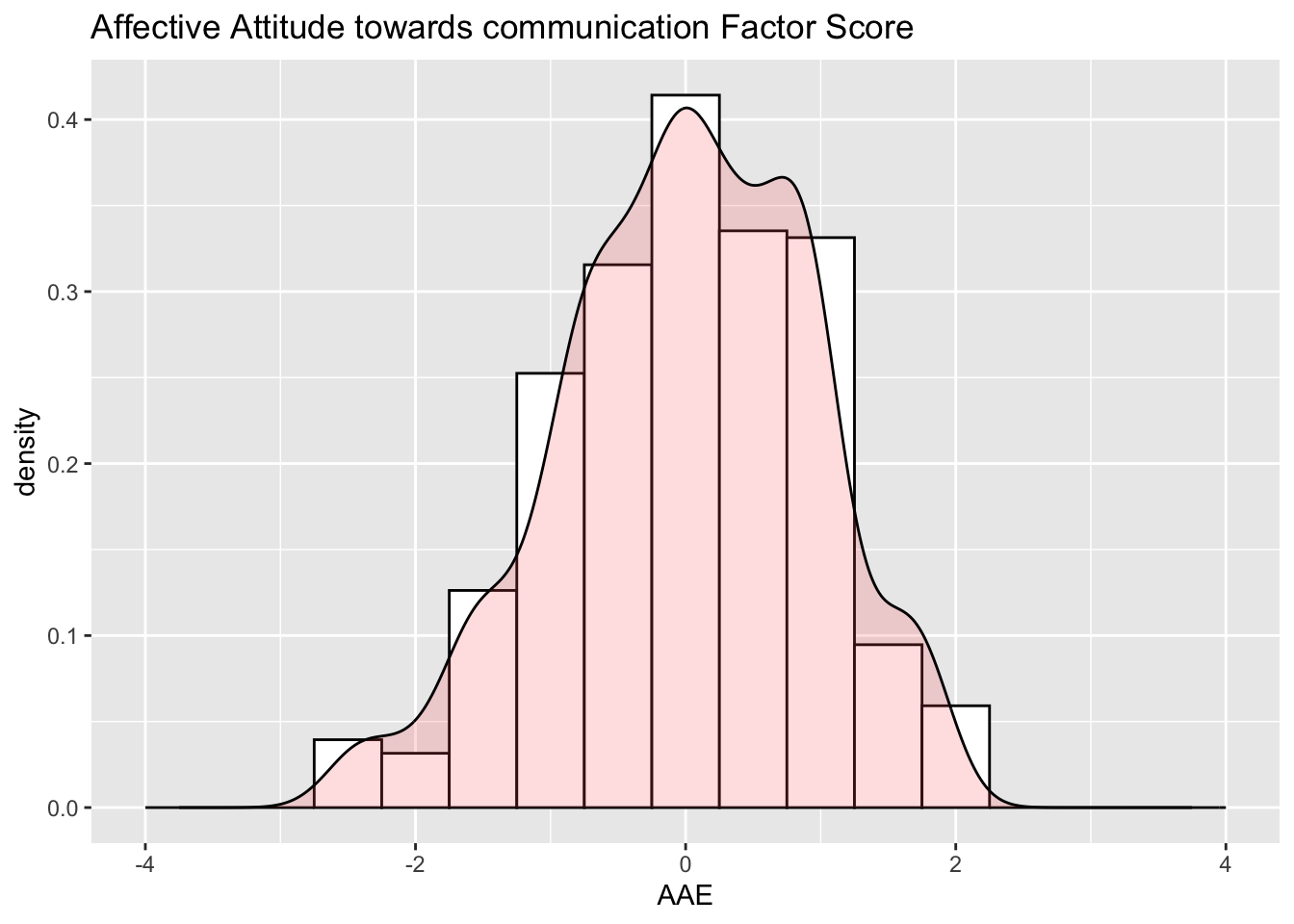
    OmegaAAE          0.830    0.017   49.000    0.000

6 Factor Scores and Distributions

The AAC factor scores have an estimated mean of 0 with a variance of 0.88 due to the effect of the prior distribution. The SE for each person’s AAC factor score is 0.347; 95% confidence interval for AAC factor score is Score \pm 2*0.347 = Score \pm 0.694. The AAE factor scores have an estimated mean of 0 with a variance of 0.881 due to the effect of the prior distribution. The SE for each person’s AAC factor score is 0.357; 95% confidence interval for AAC factor score is Score \pm 2*0.357 = Score \pm 0.714.

Factor Realiability for AAC is 0.892 and factor realibility for AAE is 0.887. Both factor reliability are larger than omega.

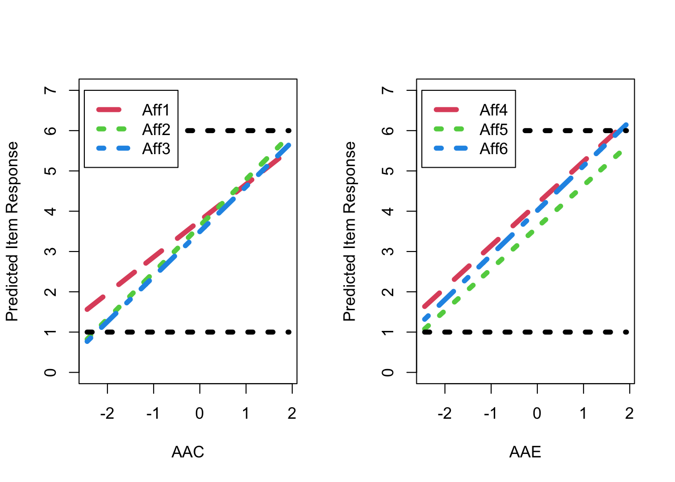
The resulting distribution of the EAP estimates of factor score as shown in Figure 1. Figure 2 shows the predicted response for each item as a linear function of the latent factor based on the estimated model parameters. As shown, for AAE factor, the predicted item response goes above the highest response option just before a latent factor score of 2 (i.e., 2 SDs above the mean), resulting in a ceiling effect for AAE factor, as also shown in Figure 1.

The extent to which the items within each factor could be seen as exchangeable was then examined via an additional set of nested model comparisons, as reported in Table 1 (for fit) and Table 2 (for comparisons of fit). Two-factor has better model fit than one-facor model. Moreover, according to chi-square difference test, two-factor is significantly better than one-factor in model fit.

      AAC       AAE 
0.8925361 0.8867031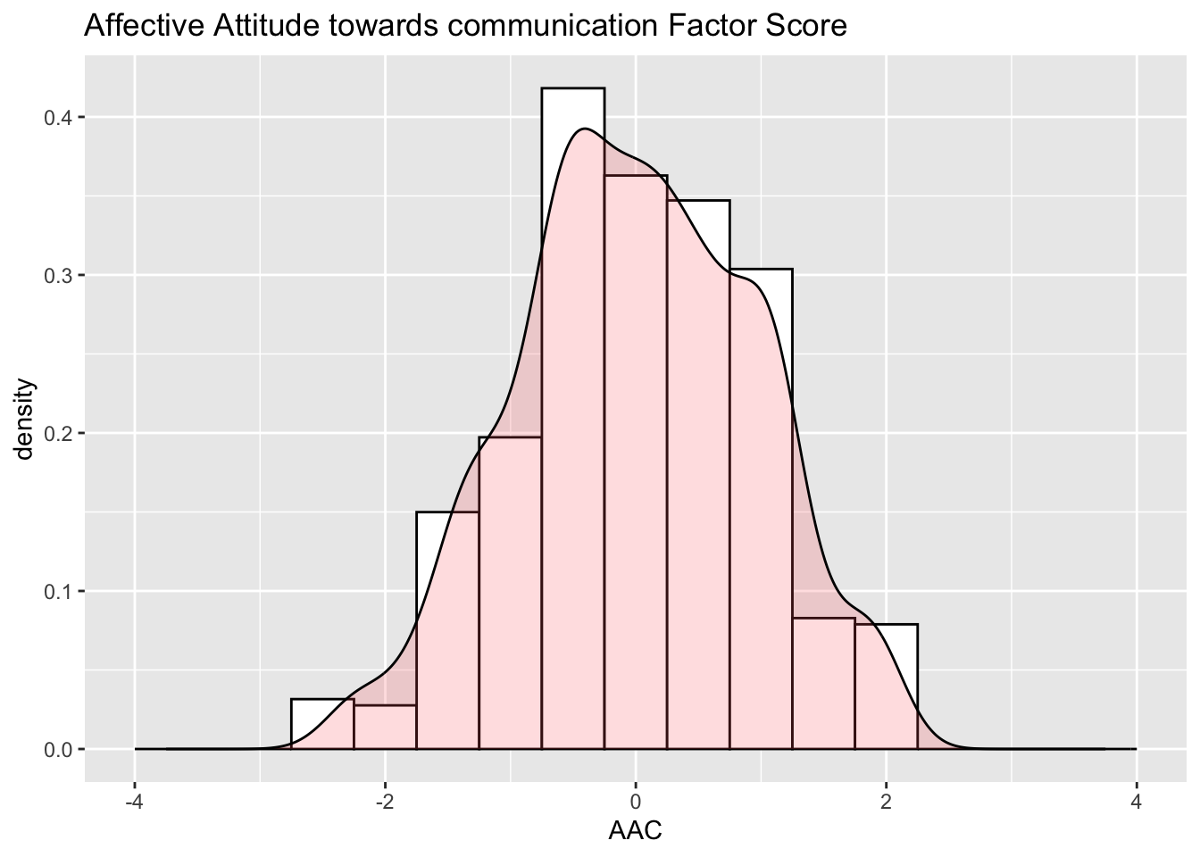

7 Figures

7.1 Figure 1 : Factor Score Distribution

7.2 Figure 2 : Expected Item Response Plots

8 Tables

8.1 Table 1: Model Fit Statistics Using MLR

	# Items	# Parameters	Scaled Chi-Square	Chi-Square Scale Factor	DF	p-value	CFI	RMSEA	RMSEA Lower	RMSEA Upper	RMSEA p-value
One-Factor	6	18	75.834	1.522	9	0.000	0.927	0.9	0.000	0.05	1.000
Two-Factor	6	19	21.512	1.503	8	0.006	0.979	0.9	0.046	0.05	0.475

8.2 Table 2: Model Comparisons

	Df	Chisq diff	Df diff	Pr(>Chisq)
One-Factor vs. Two-Factor	9	49.652	1	0

8.3 Table 3: Model Estimates

	Unstandardized		Standardized
	Estimate	SE	Estimate
Forgiveness Factor Loadings
Item 1	0.903	0.055	0.676
Item 2	1.153	0.042	0.865
Item 3	1.117	0.051	0.820
Not Unforgiveness Factor Loadings
Item 4	1.047	0.053	0.796
Item 5	1.036	0.053	0.728
Item 6	1.107	0.044	0.844
Factor Covariance
Factor Covariance	0.838	0.028	0.838
Item Intercepts
Item 1	3.765	0.059	2.818
Item 2	3.635	0.059	2.726
Item 3	3.493	0.060	2.564
Item 4	4.189	0.058	3.184
Item 5	3.604	0.063	2.534
Item 6	4.018	0.058	3.062
Item Unique Variances
Item 1	0.970	0.083	0.543
Item 2	0.449	0.057	0.253
Item 3	0.607	0.084	0.327
Item 4	0.635	0.085	0.367
Item 5	0.950	0.090	0.470
Item 6	0.497	0.061	0.288