Network psychometrics has become an alternative approach to factor analysis and item response theory in multiple fields of psychology and education, such as psychopathology, personality, measurement validation, and dimensionality determancy etc. However, individual scoring differences between psychometric network analysis and traditional psychometric modeling has not been well investigated. Some questions arise regarding individual scoring:
What will be individual scores in psychometric network analysis? Or, how can we evaluate the average level of each individuals?
If we can build individual scoring in psychometric network, what is the relationship between this scoring with factor scores.
How can we use this scoring method to evaluate measurement quality, such as reliability or validity?
To answer these questions, we first need to review how individuals are scored in factor analysis method and classical test theory. Borrowing the theoretical framework and purpose of factor scoring, we can construct the scoring method for psychometric network. Then, we can show that there are statistical relationship between network scores with factor scores. Thus, depending on the psychometric methods researchers use, they can be free to use either factor score or network score to report. They can also compute the other without constructing the other model.
Overall, the purpose of this post is to illustrate the definition, assumption, psychometric properties, usage, and interpretation of factor scores in Structural Equation Models (SEM), and how those features of factor scores compare to sum scores in Classical Test Theory (CTT). This post is inspired by Dr. Templin’s 2022 presentation.
1 Definition of Test Score
In CTT, the test score is unit of analysis of the whole test, which can be statistically expressed as:
Y_{total} = T+e
Where Y_{total} denotes test scores, T denotes true score, and e denotes error. There are some assumptions:
Items are assumed exchangeable;
Expected value of e is 0;
Error e is expected to be uncorrelated with true score T
2 Scoring of Classical test theory
In classical test theory (CTT), the test score is construct as sum of item scores. CTT assumes that there is a true score exists that reflect the true ability of test takers and the observed sum scores of each individual is a combination of true score and random error.
Y_{total} = T + e
Where Y_{total} denotes a vector of observed sum scores of respondents, T denotes a vector of true scores of respondents, and e denotes the random error for respondents. True scores and random errors are independent.
2.1 CTT-based reliability
Multiple reliability coefficients have been proposed in previous literature. Each reliability has their advantages and disadvantages. Let’s take the average iter-item correlation as one example. Average iter-item correlation is computed as the proportion of variance in the sum score that is due to variation in the latent trait or true score.
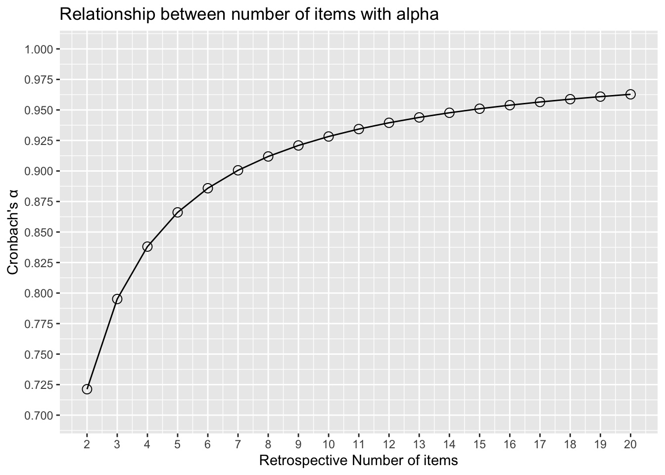
One estimate of the internal consistency reliability of a test is Cronbach’s \alpha, which summarizes the average item-test correlation.
The standard Cronbach’s \alpha is .93. The average Iter-Item Correlation is .564. Ideally, the average inter-item correlation for a set of items should be between .20 and .40, suggesting that while the items are reasonably homogenous, they do contain sufficiently unique variance so as to not be isomorphic with each other (Piedmont, 2014).
library(greekLetters) tibble(nItems =2:20, alpha = nItems*rho / (1+ (nItems-1)*rho )) |>ggplot() +aes(x = nItems, y = alpha) +geom_point(size =3, shape =1) +geom_path(group =1) +scale_x_continuous(breaks =2:20) +scale_y_continuous(breaks =seq(0.7, 1, .025), limits =c(0.7, 1)) +labs(x ='Retrospective Number of items', y =paste0("Cronbach's ", greeks('alpha')),title ='Relationship between number of items with alpha')
3 Scoring of Factor Analysis
In factor analysis, factor scores are computed using parameters of CFA, i.e., unique variances (\Psi), factor loadings (\Lambda) and factor correlations (\Phi). In most modern statistical software (i.e., lavaan or Mplus), factor scores are estimated by multivariate methods that use various aspects of the reduced or unreduced correlation matrix and factor analysis coefficients (Brown, 2015). A frequently used method of estimating factor scores is Thurston’s (1935) least squared regression approach, although several other strategies have been developed (e.g., Bartlett, 1937; Harman, 1976; McDonald, 1982).
Brown, T. A. (2015). Confirmatory factor analysis for applied research: Second edition. Guilford Press.
Ferrando, P. J., & Lorenzo-Seva, U. (2018). Assessing the Quality and Appropriateness of Factor Solutions and Factor Score Estimates in Exploratory Item Factor Analysis. Educational and Psychological Measurement, 78(5), 762–780. https://doi.org/10.1177/0013164417719308
Where \boldsymbol{\theta_i} and \boldsymbol{Y}_i are factor score estimates and item responses for individual i, respectively; \Phi is the factor correlation matrix (for example, for single factor model, \Phi is 1 \times 1 matrix ), \Psi is J \times J unique variances of items, and \Lambda is the pattern loading matrix. \boldsymbol{S} is the factor loading structure matrix with the size I \times P where I denotes number of item and P denotes number of latent factors. For unidimensional structure, \boldsymbol{S} = \boldsymbol{\Lambda}.
To derive the Thurston’s method, we can first partition joint distribution of all I items and K factor scores as
f(\boldsymbol{\theta, Y}) = f(\begin{bmatrix}\Theta\\Y\end{bmatrix}) \\
= N_{I+K}(\begin{bmatrix}\mu_\Theta \\ \mu+\Lambda'\mu_\Theta \end{bmatrix},
\begin{bmatrix}
\Phi\Lambda' \space\space\space\space\space\space\space\space\space \Phi \\
\Lambda\Phi\Lambda'+\Psi \space\space \Lambda\Phi
\end{bmatrix})
Based on relationship between conditional distribution of f(\theta|Y) and joint distribution of f(Y, \theta):
Where \mu_1 and \mu_2 are mean components of partitioned joint distribution, and \Sigma_{12} and \Sigma_{22} are [1,2] and [2,2] elements of variance components of partitioned joint distribution.Then,
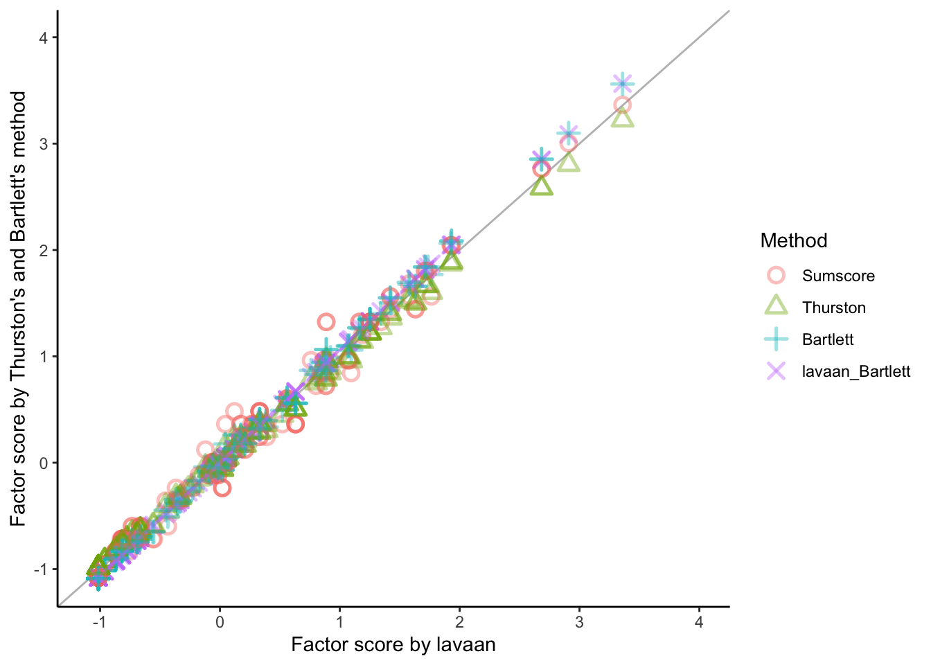
Using the consipiracy theory data, we can calculate the factor scores based on the equation mention above using Thurston’s method and compare to the estimated factor score by lavaan.
lavaan code
model2 <-' F1 =~ PolConsp1+PolConsp2+PolConsp3+PolConsp4+PolConsp5+PolConsp6+PolConsp7+PolConsp8+PolConsp9+PolConsp10'fit2 =cfa(model = model2, data = itemResp_std, std.lv =TRUE)summary(fit2)
lavaan 0.6-19 ended normally after 20 iterations

  Estimator                                         ML
  Optimization method                           NLMINB
  Number of model parameters                        20

  Number of observations                           177

Model Test User Model:

  Test statistic                               120.975
  Degrees of freedom                                35
  P-value (Chi-square)                           0.000

Parameter Estimates:

  Standard errors                             Standard
  Information                                 Expected
  Information saturated (h1) model          Structured

Latent Variables:
                   Estimate  Std.Err  z-value  P(>|z|)
  F1 =~
    PolConsp1         0.627    0.069    9.127    0.000
    PolConsp2         0.755    0.065   11.677    0.000
    PolConsp3         0.706    0.066   10.647    0.000
    PolConsp4         0.734    0.065   11.234    0.000
    PolConsp5         0.871    0.060   14.528    0.000
    PolConsp6         0.865    0.060   14.367    0.000
    PolConsp7         0.735    0.065   11.244    0.000
    PolConsp8         0.865    0.060   14.361    0.000
    PolConsp9         0.730    0.065   11.154    0.000
    PolConsp10        0.615    0.069    8.893    0.000

Variances:
                   Estimate  Std.Err  z-value  P(>|z|)
   .PolConsp1         0.601    0.067    9.030    0.000
   .PolConsp2         0.425    0.049    8.634    0.000
   .PolConsp3         0.496    0.056    8.828    0.000
   .PolConsp4         0.455    0.052    8.724    0.000
   .PolConsp5         0.236    0.031    7.540    0.000
   .PolConsp6         0.246    0.032    7.643    0.000
   .PolConsp7         0.455    0.052    8.723    0.000
   .PolConsp8         0.247    0.032    7.646    0.000
   .PolConsp9         0.461    0.053    8.740    0.000
   .PolConsp10        0.617    0.068    9.055    0.000
    F1                1.000
fs = fs |>pivot_longer(c(lavaan_Bartlett, Sumscore, Thurston, Bartlett), names_to ="Method", values_to ="Score") |>mutate(Method =factor(Method, levels =c("Sumscore", "Thurston", "Bartlett", "lavaan_Bartlett")))ggplot(fs) +geom_abline(aes(slope =1, intercept =0), color ="grey") +geom_point(aes(x = lavaan_regression, y = Score, color = Method, shape = Method), size =3, alpha = .4, stroke =1.3) +labs(x ="Factor score by lavaan", y ="Factor score by Thurston's and Bartlett's method") +scale_shape_manual(values =1:4) +scale_y_continuous(limits =c(-1.1, 4)) +scale_x_continuous(limits =c(-1.1, 4)) +theme_classic()
3.2 Mplus
In Mplus, latent factor score estimation can have varied methods under two condition: (1) when individual level factor scores are of interests, factor scores are estimated based on either Maximum-likelihood estimators or Bayes estimators; (2) when factor scores are used for secondary analysis (dependent variables of regression models), factor scores are viewed as one type of imputed values, thus they are also known as plausible values and estimated by Bayesian imputation and Rubin’s (1978) method (Asparouhov & Muthen, 2010; Rubin, 1978; von Davier et al., 2009).
Rubin, D. B. (1978). Multiple imputation for nonresponse in surveys - a phenomenological bayesian approach to nonresponse. J. Wiley & Sons, New York.
Under the first condition, according to simulation study of Asparouhov & Muthen (2010), using ML estimators and small sample size, standardized errors for factor scores is underestimated. Another finding is that the larger the absolute factor score value is the larger the standard error is. This is because large absolute factor score values are generally in the tail of the factor score distribution, i.e., in a region with fewer observations.
With continuous variable, Mplus estimates factor scores as the maximum of posterior distribution of the factor (also called the Maximum A Posterior method), which is the same as the Regression Method for factor score estimation (Asparouhov & Muthen, 2010; Skrondal & Laake, 2001). It should be noted that, with this method, using factor scores as predictors given unbiased regression slopes, but using factor scores as dependent variables gives biased slopes. With categorical variables and the maximum-likelihood estimator, Mplus estimates factor scores as the expected value of the posterior distribution of the factor, which is also called the Expected A Posteriori (EAP) method.
Asparouhov, T., & Muthen, B. (2010). Plausible values for latent variables using mplus.
Relationship between factor score and network score
The official paper will show both factor score and network score of unidimensional factor analysis is a special case of general scoring form when weight matrix is factor loadings or centrality measures.
Correlation between factor scores and network scores
For network model,
\hat \Sigma = \Delta(I-\Omega)^{-1}\Delta
where \Omega is a edge weight matrix or a standardized partial correlation matrix with diagonal elements as zeros, \Delta is the diagonal matrix with element \delta_{jj} =\kappa_{jj}^{-\frac{1}{2}}. That is,
\Delta = \text{diag}(\hat K)^{-\frac12}
We can derive the above Equation by assuming the precision matrix \kappa and partial correlation \omega_{jk} has following relationship:
\boldsymbol{\hat\eta_i= W \Delta^{-1}(I-\Omega)\Delta^{-1} Y_i}
\tag{2} Where \boldsymbol{W} is a 1 \times J weight matrix suggesting the “importance” of items.
Thus, as shown in Equation 2, we can conclude that when \boldsymbol{W \approx \Lambda}, then \boldsymbol{\hat\eta \approx \hat\theta}; when \boldsymbol{W \approx S}, then \boldsymbol{\hat\eta \approx \hat{FS}}
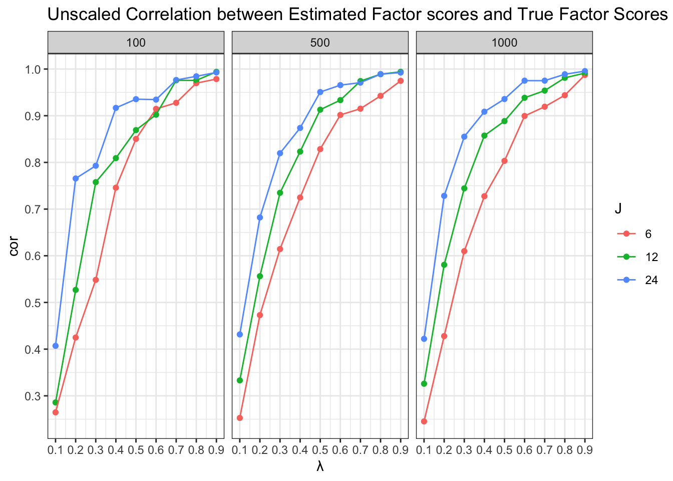
4 Correlation between estimated factor scores and true factor scores
When item responses and factor scores are standardized, based on Thurston’s regression method (see Equation 1), the estimated factor scores are:
The relationship between estimated factor scores and true factor scures is a simple linear regression with \Lambda'(\Lambda\Lambda'+\Psi)^{-1}\Lambda as the estimated linear slope.
For simple linear regression Y=b_0+b_1X, the Pearson’s correlation is r = b_1 * \frac{S_X}{S_Y}. Then, when both \hat \theta_i and \theta_i^T are normal distributed, then the correlation between estimated and true factor score is as:
---title: 'Sum Score, Factor Score, and Reliability'author: 'Jihong Zhang'date: 'Mar 12 2024'image: "Sim_FactorScore_NetworkScore_Correlation.png"categories: - Scoring - Reliability - CTT - Factor Analysisexecute: warning: false message: falsecitation: trueformat: html: code-fold: true code-line-numbers: falsebibliography: references.bibcsl: apa.csl---Network psychometrics has become an alternative approach to factor analysis and item response theory in multiple fields of psychology and education, such as psychopathology, personality, measurement validation, and dimensionality determancy etc. However, individual scoring differences between psychometric network analysis and traditional psychometric modeling has not been well investigated. Some questions arise regarding individual scoring:1. What will be individual scores in psychometric network analysis? Or, how can we evaluate the average level of each individuals?2. If we can build individual scoring in psychometric network, what is the relationship between this scoring with factor scores.3. How can we use this scoring method to evaluate measurement quality, such as reliability or validity?To answer these questions, we first need to review how individuals are scored in factor analysis method and classical test theory. Borrowing the theoretical framework and purpose of factor scoring, we can construct the scoring method for psychometric network. Then, we can show that there are statistical relationship between network scores with factor scores. Thus, depending on the psychometric methods researchers use, they can be free to use either factor score or network score to report. They can also compute the other without constructing the other model.Overall, the purpose of this post is to illustrate the definition, assumption, psychometric properties, usage, and interpretation of factor scores in Structural Equation Models (SEM), and how those features of factor scores compare to sum scores in Classical Test Theory (CTT). This post is inspired by Dr. Templin's [2022 presentation](https://jonathantemplin.com/wp-content/uploads/2022/10/sem15pre906_lecture11.pdf).## Definition of Test ScoreIn CTT, the test score is unit of analysis of the whole test, which can be statistically expressed as:$$Y_{total} = T+e$$Where $Y_{total}$ denotes test scores, $T$ denotes true score, and $e$ denotes error. There are some assumptions:1. Items are assumed exchangeable;2. Expected value of $e$ is 0;3. Error $e$ is expected to be uncorrelated with true score $T$## Scoring of Classical test theoryIn classical test theory (CTT), the test score is construct as sum of item scores. CTT assumes that there is a true score exists that reflect the true ability of test takers and the observed sum scores of each individual is a combination of true score and random error.$$Y_{total} = T + e$$Where $Y_{total}$ denotes a vector of observed sum scores of respondents, $T$ denotes a vector of true scores of respondents, and $e$ denotes the random error for respondents. True scores and random errors are independent.### CTT-based reliabilityMultiple reliability coefficients have been proposed in previous literature. Each reliability has their advantages and disadvantages. Let's take the average iter-item correlation as one example. Average iter-item correlation is computed as the proportion of variance in the sum score that is due to variation in the latent trait or true score.We can derive the reliability as following:$$\text{Var}(Y_{total}) = \text{Var}(T+e) = \text{Var}(T)+\text{Var}(e)+2\text{Cov}(T,e)$$But, since T and e are assumed independent $\text{Cov}(T, e) = 0$, so,$$\text{Var}(Y_{total}) = \text{Var}(T)+\text{Var}(e)$$Then, reliability can be computed as:$$\rho = \frac{\text{Var}(T)}{\text{Var}(Y)} = \frac{\text{Var}(T)}{\text{Var}(T)+\text{Var}(e)} $$Where,- $\text{Var}(T)$ is variance of true score and could be interpreted as variability in the latent trait in the context of factor analysis.- $\text{Var}(e)$ is variance of error, and could be interpreted as measurement error#### Mini exampleUsing a 10-item example with each having 1-5 scale.```{r}#| code-fold: true#| code-summary: 'Data Read-in'library(tidyverse)library(here)library(kableExtra)library(psych)dat_path <-'posts/Lectures/2024-01-12-syllabus-adv-multivariate-esrm-6553/Lecture07/Code'conspiracy <-read.csv(here(dat_path, 'conspiracies.csv'))itemResp <- conspiracy |>select(starts_with('PolConsp'))conspiracy |>mutate(ID =1:177) |>pivot_longer(starts_with('PolConsp'), names_to ='Item', values_to ='Resp') |>mutate(Item =factor(Item, paste0('PolConsp', 1:10))) |>group_by(Item) |>summarise(Mean =mean(Resp),SD =sd(Resp),Min =min(Resp),Max =max(Resp),Skew = psych::skew(Resp) ) |>kable(digits =3)```One estimate of the internal consistency reliability of a test is <mark>Cronbach's $\alpha$</mark>, which summarizes the average item-test correlation.The standard Cronbach's $\alpha$ is .93. The average Iter-Item Correlation is .564. Ideally, the average inter-item correlation for a set of items should be between .20 and .40, suggesting that while the items are reasonably homogenous, they do contain sufficiently unique variance so as to not be isomorphic with each other [@piedmont2014].```{r}#| code-summary: "Reliability by psych package"kable(alpha(itemResp)$total, digits =3)```Using factor analysis and `lavaan`, we can reproduce average inter-item correlations assuming items are tau-equavalent:- Item responses are standardized (mean as 0, variance as 1)- Factor loadings are constrained to be equal as 1- Residual variances of items are constrained to be equalThen, iter-item correlation and Cronbach's alpha can be computed as:$$\rho = \frac{\text{Var}(\theta)}{\text{Var}(\theta)+\text{Var}(\psi)}$$$$\alpha = \frac{N\rho}{\sigma^2 +(N-1)\rho}$$where N is sample size, $\rho$ is average iter-item correlation, and $\sigma^2$ are average item variances and equal to 1 if items are standardized.```{r}#| code-summary: 'iter-item correlation by lavaan'library(lavaan)itemResp_std <- itemResp |>mutate(across(everything(), scale))unifac_model <-'F1 =~ 1*PolConsp1+1*PolConsp2+1*PolConsp3+1*PolConsp4+1*PolConsp5+1*PolConsp6+1*PolConsp7+1*PolConsp8+1*PolConsp9+1*PolConsp10PolConsp1 ~~equal("e1")*PolConsp1PolConsp2 ~~equal("e1")*PolConsp2PolConsp3 ~~equal("e1")*PolConsp3PolConsp4 ~~equal("e1")*PolConsp4PolConsp5 ~~equal("e1")*PolConsp5PolConsp6 ~~equal("e1")*PolConsp6PolConsp7 ~~equal("e1")*PolConsp7PolConsp8 ~~equal("e1")*PolConsp8PolConsp9 ~~equal("e1")*PolConsp9PolConsp10~~equal("e1")*PolConsp10'fit =cfa(model = unifac_model, data = itemResp_std, std.lv =FALSE)# summary(fit)Var_F1 =as.numeric(coef(fit)['F1~~F1'])Var_errors=as.numeric(coef(fit)[1])rho = Var_F1 / (Var_F1 + Var_errors) # reliability rho # average iter-item correlation``````{r}#| code-summary: "Cronbach's alpha by lavaan"Cron_alpha =10*rho / (1+ (10-1)*rho )Cron_alpha # Cronbach's alpha```Cronbach's alpha is related to number of items:```{r}#| code-summary: 'Correlation between alpha and test length'#| code-fold: true#| fig-align: centerlibrary(greekLetters) tibble(nItems =2:20, alpha = nItems*rho / (1+ (nItems-1)*rho )) |>ggplot() +aes(x = nItems, y = alpha) +geom_point(size =3, shape =1) +geom_path(group =1) +scale_x_continuous(breaks =2:20) +scale_y_continuous(breaks =seq(0.7, 1, .025), limits =c(0.7, 1)) +labs(x ='Retrospective Number of items', y =paste0("Cronbach's ", greeks('alpha')),title ='Relationship between number of items with alpha')```## Scoring of Factor AnalysisIn factor analysis, factor scores are computed using parameters of CFA, i.e., unique variances ($\Psi$), factor loadings ($\Lambda$) and factor correlations ($\Phi$). In most modern statistical software (i.e., lavaan or Mplus), factor scores are estimated by multivariate methods that use various aspects of the reduced or unreduced correlation matrix and factor analysis coefficients [@brownConfirmatoryFactorAnalysis2015]. A frequently used method of estimating factor scores is Thurston's (1935) least squared regression approach, although several other strategies have been developed (e.g., Bartlett, 1937; Harman, 1976; McDonald, 1982).For confirmatory factor analysis that is identified, the scoring method discussed by Thurston (1935) and Thomson (1934) has the closed form [@ferrando2018; @skrondalRegressionFactorScores2001]:$$\text{EAP}(\boldsymbol{\theta}_i) = \boldsymbol{\Phi}\boldsymbol{\Lambda}'\boldsymbol{R}^{-1}\boldsymbol{Y}_i=\boldsymbol{S}'\boldsymbol{R}^{-1}\boldsymbol{Y}_i$$ {#eq-thurston}and $\boldsymbol{R}$ is the the estimated item covaraince matrix:$$\boldsymbol{R} = \boldsymbol{\Lambda}\boldsymbol{\Phi}\boldsymbol{\Lambda}'+\boldsymbol{\Psi}$$Where $\boldsymbol{\theta_i}$ and $\boldsymbol{Y}_i$ are factor score estimates and item responses for individual $i$, respectively; $\Phi$ is the factor correlation matrix (for example, for single factor model, $\Phi$ is 1 $\times$ 1 matrix ), $\Psi$ is $J \times J$ unique variances of items, and $\Lambda$ is the pattern loading matrix. $\boldsymbol{S}$ is the factor loading structure matrix with the size $I \times P$ where $I$ denotes number of item and $P$ denotes number of latent factors. For unidimensional structure, $\boldsymbol{S} = \boldsymbol{\Lambda}$.To derive the Thurston's method, we can first partition joint distribution of all $I$ items and $K$ factor scores as$$f(\boldsymbol{\theta, Y}) = f(\begin{bmatrix}\Theta\\Y\end{bmatrix}) \\= N_{I+K}(\begin{bmatrix}\mu_\Theta \\ \mu+\Lambda'\mu_\Theta \end{bmatrix},\begin{bmatrix}\Phi\Lambda' \space\space\space\space\space\space\space\space\space \Phi \\\Lambda\Phi\Lambda'+\Psi \space\space \Lambda\Phi\end{bmatrix})$$ Based on relationship between conditional distribution of $f(\theta|Y)$ and joint distribution of $f(Y, \theta)$:$$\boldsymbol{\mu^*=\mu_1+\Sigma_{12}\Sigma_{22}^{-1}(Y-\mu_2)}$$Where $\mu_1$ and $\mu_2$ are mean components of partitioned joint distribution, and $\Sigma_{12}$ and $\Sigma_{22}$ are \[1,2\] and \[2,2\] elements of variance components of partitioned joint distribution.Then,$$f(\boldsymbol{\theta|Y}) = \mu_\Theta + \Phi\Lambda'(\Lambda\Phi\Lambda'+\Psi)^{-1}(Y'-(\mu+\Lambda'\mu_\Theta))$$Assume factor scores and item responses are standardized, $\mu_\Theta = 0$ and $\mu = 0$, then this is equivalent to @eq-thurston.Alternatively, using [Bartlett's (1937, 1938)]{.underline} method [@skrondalRegressionFactorScores2001], factor scores can be estimated as:$$\text{EAP}(\boldsymbol{\theta_i}) = \boldsymbol{(\Lambda'\Psi^{-1}\Lambda)^{-1}\Lambda'\Psi^{-1}Y_i}$$### lavaanUsing the consipiracy theory data, we can calculate the factor scores based on the equation mention above using Thurston's method and compare to the estimated factor score by `lavaan`.```{r}#| code-summary: 'lavaan code'model2 <-' F1 =~ PolConsp1+PolConsp2+PolConsp3+PolConsp4+PolConsp5+PolConsp6+PolConsp7+PolConsp8+PolConsp9+PolConsp10'fit2 =cfa(model = model2, data = itemResp_std, std.lv =TRUE)summary(fit2)``````{r}#| code-summary: "Thurston's and Bartlett's method"## extract factor loadings and unique varianceslambdas =as.numeric(coef(fit2)[paste0("F1=~PolConsp", 1:10)])Lambda =matrix(lambdas, ncol =1)psis =as.numeric(coef(fit2)[paste0("PolConsp", 1:10, "~~PolConsp", 1:10)])Psi =diag(sqrt(psis))Phi =diag(1)## Estimated Structural correlation matrixR = Lambda %*% Phi %*%t(Lambda) + Psi## Thurston's method# FNS_influence <- Y %*% rowSums(precision_mat) # calculate FNS based on expected influence# LNS_influence <- Y %*% precision_mat %*% rowSums(precision_mat) # calculate LNS based on expected inlfuenceTheta_thurston =as.numeric(diag(1) %*%t(Lambda) %*%solve(R) %*%t(itemResp_std))## Bartlett's methodTheta_bartlett =as.numeric(solve(t(Lambda) %*%solve(Psi) %*% Lambda) %*%t(Lambda) %*%solve(Psi) %*%t(itemResp_std))Theta_lavaan_regression =as.numeric(lavPredict(fit2, method ='regression'))Theta_lavaan_Bartlett =as.numeric(lavPredict(fit2, method ='Bartlett'))```We can find that Thurston's method is consistent with `lavaan` 's output of factor scores:```{r}#| code-summary: 'Comparison'fs =tibble(lavaan_regression = Theta_lavaan_regression,lavaan_Bartlett = Theta_lavaan_Bartlett,Thurston = Theta_thurston,Bartlett = Theta_bartlett,Sumscore =as.numeric(scale(rowSums(itemResp)))) cor(fs)fs = fs |>pivot_longer(c(lavaan_Bartlett, Sumscore, Thurston, Bartlett), names_to ="Method", values_to ="Score") |>mutate(Method =factor(Method, levels =c("Sumscore", "Thurston", "Bartlett", "lavaan_Bartlett")))ggplot(fs) +geom_abline(aes(slope =1, intercept =0), color ="grey") +geom_point(aes(x = lavaan_regression, y = Score, color = Method, shape = Method), size =3, alpha = .4, stroke =1.3) +labs(x ="Factor score by lavaan", y ="Factor score by Thurston's and Bartlett's method") +scale_shape_manual(values =1:4) +scale_y_continuous(limits =c(-1.1, 4)) +scale_x_continuous(limits =c(-1.1, 4)) +theme_classic()```### MplusIn Mplus, latent factor score estimation can have varied methods under two condition: (1) when individual level factor scores are of interests, factor scores are estimated based on either Maximum-likelihood estimators or Bayes estimators; (2) when factor scores are used for secondary analysis (dependent variables of regression models), factor scores are viewed as one type of imputed values, thus they are also known as plausible values and estimated by Bayesian imputation and Rubin's (1978) method [@rubinMultipleImputationNonresponse1978; @asparouhovPlausibleValuesLatent2010; @vondavierWhatArePlausible2009].Under the first condition, according to simulation study of @asparouhovPlausibleValuesLatent2010, [using ML estimators and small sample size]{.underline}, standardized errors for factor scores is underestimated. Another finding is that the larger the absolute factor score value is the larger the standard error is. This is because large absolute factor score values are generally in the tail of the factor score distribution, i.e., in a region with fewer observations.With continuous variable, Mplus estimates factor scores as the maximum of posterior distribution of the factor (also called the *Maximum A Posterior* method), which is the same as the Regression Method for factor score estimation [@asparouhovPlausibleValuesLatent2010; @skrondalRegressionFactorScores2001]. It should be noted that, with this method, using factor scores as predictors given unbiased regression slopes, but using factor scores as dependent variables gives biased slopes. With categorical variables and the maximum-likelihood estimator, Mplus estimates factor scores as the expected value of the posterior distribution of the factor, which is also called the Expected A Posteriori (EAP) method.::: callout-note## Relationship between factor score and network scoreThe official paper will show both factor score and network score of unidimensional factor analysis is a special case of general scoring form when weight matrix is factor loadings or centrality measures.:::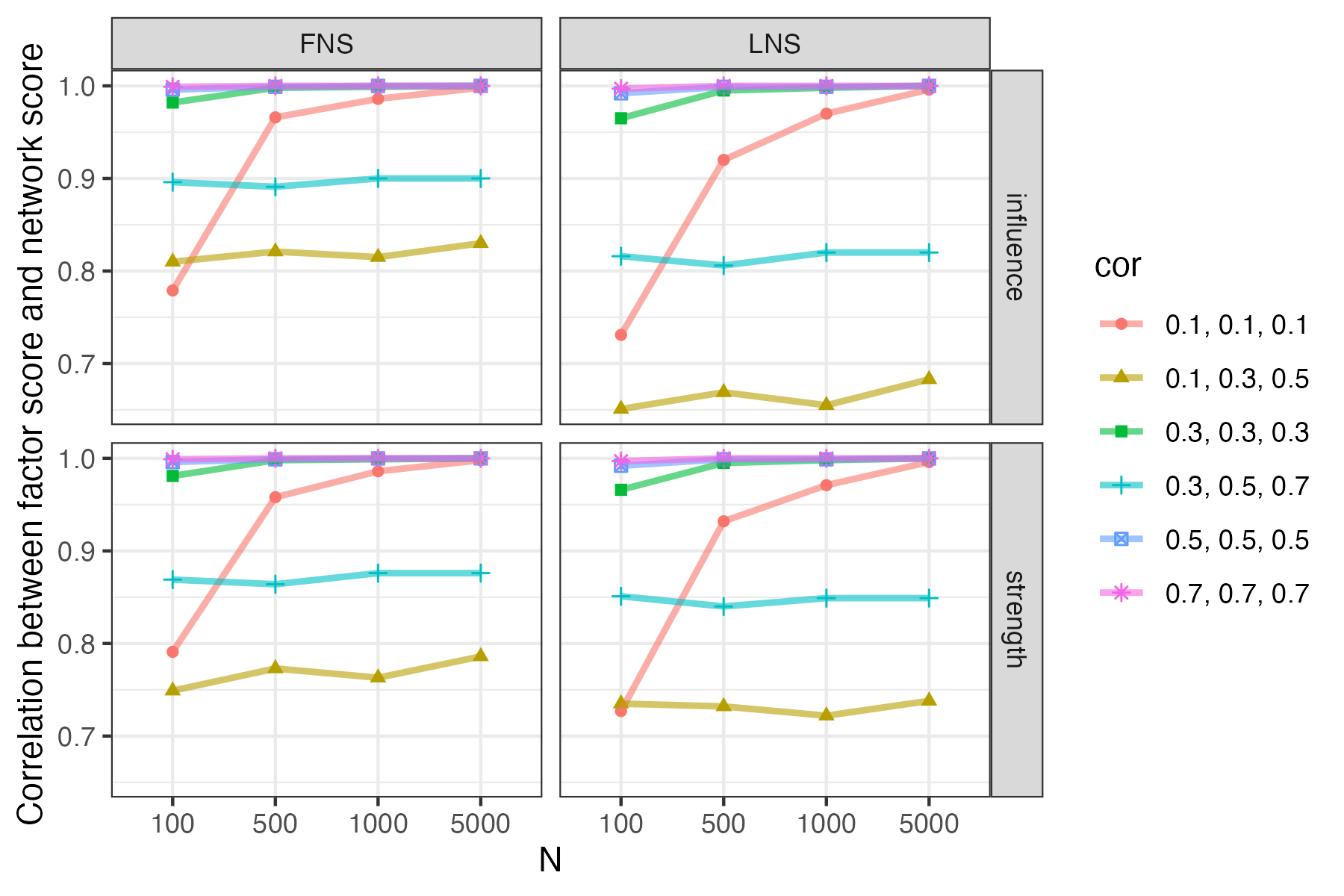{.preview-image fig-align="center"}For network model,$$\hat \Sigma = \Delta(I-\Omega)^{-1}\Delta$$where $\Omega$ is a edge weight matrix or a standardized partial correlation matrix with diagonal elements as zeros, $\Delta$ is the diagonal matrix with element $\delta_{jj} =\kappa_{jj}^{-\frac{1}{2}}$. That is,$$\Delta = \text{diag}(\hat K)^{-\frac12}$$We can derive the above Equation by assuming the precision matrix $\kappa$ and partial correlation $\omega_{jk}$ has following relationship:$$\omega_{jk} = -\frac{\kappa_{jk}}{\sqrt{\kappa_{jj}}\sqrt{\kappa_{kk}}}$$Then, since the diagnal elements of matrix $\Omega$ are zeros, it is easy to show that$$\hat K = \text{diag}{(\hat K)}^{\frac12}(I-\Omega)\text{diag}{(\hat K)}^{\frac12}$$$$\hat \Sigma = \hat K^{-1} = \text{diag}{(\hat K)}^{-\frac12}(I-\Omega)^{-1}\text{diag}{(\hat K)}^{-\frac12}$$For factor analysis,$$\hat \Sigma = \boldsymbol{\Lambda \Phi \Lambda'+\Psi}$$We can show that$$(I-\Omega)^{-1} = \Delta^{-1}(\boldsymbol{\Lambda \Phi \Lambda'+\Psi})\Delta^{-1}$$Thus,$$I - \Omega = \Delta(\boldsymbol{\Lambda \Phi \Lambda'+\Psi})^{-1}\Delta$$Based on @eq-thurston Thurston's regression method, we know that$$\boldsymbol{\hat \theta_i = \Lambda'(\Lambda \Phi \Lambda'+\Psi)^{-1}Y_i \\= \Lambda' \Delta^{-1}(I-\Omega)\Delta^{-1}Y_i}$$Then, if we set general scoring formular as$$\boldsymbol{\hat\eta_i= W \Delta^{-1}(I-\Omega)\Delta^{-1} Y_i}$$ {#eq-generalform} Where $\boldsymbol{W}$ is a $1 \times J$ weight matrix suggesting the "importance" of items.Thus, as shown in @eq-generalform, we can conclude that when $\boldsymbol{W \approx \Lambda}$, then $\boldsymbol{\hat\eta \approx \hat\theta}$; when $\boldsymbol{W \approx S}$, then $\boldsymbol{\hat\eta \approx \hat{FS}}$## Correlation between estimated factor scores and true factor scoresWhen item responses and factor scores are standardized, based on Thurston's regression method (see @eq-thurston), the estimated factor scores are:$$\hat\theta_i =\Lambda'R^{-1}Y_i \\=\Lambda'(\Lambda\Lambda'+\Psi)^{-1}(\Lambda\theta_i^T+e_i) \\=\Lambda'(\Lambda\Lambda'+\Psi)^{-1}\Lambda\theta_i^T+\Lambda'(\Lambda\Lambda'+\Psi)^{-1}e_i$$The relationship between estimated factor scores and true factor scures is a [**simple linear regression**]{.underline} with $\Lambda'(\Lambda\Lambda'+\Psi)^{-1}\Lambda$ as the estimated linear slope.For simple linear regression $Y=b_0+b_1X$, the Pearson's correlation is $r = b_1 * \frac{S_X}{S_Y}$. Then, when both $\hat \theta_i$ and $\theta_i^T$ are normal distributed, then the correlation between estimated and true factor score is as:$$r_{\hat\theta\theta^T}^{Turston}= \Lambda'(\Lambda'\Lambda+\Psi)^{-1}\Lambda\frac{S_{\theta^T}}{S_{\hat\theta}} $$Using R, we can estimate "unscaled" correlation for $\lambda = .7$ and $J = 6$ as```{r}#| fig-height: 10#| code-fold: falsesuppressMessages(library(tidyverse))set.seed(1234)corr_true_est_theta <-function(lambda, J, N) { Lambdas =matrix(rep(lambda, J), ncol =1) Psi =diag(1- lambda^2, J) corr <-t(Lambdas) %*%solve(Lambdas %*%t(Lambdas) + Psi) %*% Lambdas true_fac_score =rnorm(N, 0, 1) Y =t(Lambdas %*% true_fac_score) + mvtnorm::rmvnorm(N, sigma = Psi) est_fac_score =as.numeric(t(Lambdas) %*%solve(Lambdas %*%t(Lambdas) + Psi) %*%t(Y)) corr = corr * (sd(true_fac_score)/sd(est_fac_score)) corr}corr_true_est_theta(lambda =0.7, J =6, N =500)``````{r}#| fig-height: 5#| fig-align: center#| code-fold: falsedat <-expand.grid(lambda=seq(.1,.9,.1), J =c(6, 12 , 24), N =c(100, 500, 1000)) |>as.data.frame() |>rowwise() |>mutate(cor =corr_true_est_theta(lambda = lambda, J = J, N = N),J =factor(J, levels =c(6, 12 , 24)),N =factor(N, levels =c(100, 500, 1000)))ggplot(dat) +geom_point(aes(x=lambda, y = cor, col = J)) +geom_path(aes(x=lambda, y = cor, group = J, col = J)) +scale_x_continuous(breaks =seq(.1,.9,.1)) +scale_y_continuous(breaks =seq(.1, 1,.1)) +facet_wrap(~ N) +labs(x = greekLetters::greeks("lambda"), title ="Unscaled Correlation between Estimated Factor scores and True Factor Scores") +theme_bw()```