A dataset containing items that measure Post-traumatic stress disorder symptoms (Armour et al. 2017). There are 20 variables (p) and 221 observations (n).
Estimation of Partial Correlation Matrix
The GGM can be estimated using estimate function with some important arguments:
type: could be continuous, binary, ordinal, or mixed
iter: Number of iterations (posterior samples; defaults to 5000).
prior_sd: Scale of the prior distribution, approximately the standard deviation of a beta distribution (defaults to 0.50).
Click to see the code
library(BGGM)library(tidyverse) # for ggplot2 and dplyrlibrary(psychonetrics) # the frequentist way for GGM# dataY <- ptsd[, 1:5] +1# add + 1 to make sure the ordinal variable start from '1'# ordinal modelfit <-estimate(Y, type ='ordinal', analytic =FALSE)fit_cont <-estimate(Y, type ='continuous', analytic =FALSE)#summary(fit)pcor_mat(fit)
freqEst <-pcor_to_df(getmatrix(mod_saturated_ord, 'omega')) freqEst_cont <-pcor_to_df(getmatrix(mod_saturated_cont, 'omega')) # transform partial corr. mat. of BGGM into df.BayesEst <-pcor_to_df(pcor_mat(fit))BayesEst_cont <-pcor_to_df(pcor_mat(fit_cont)) combEst <-rbind( freqEst |>mutate(Type ='psychonetrics_ord'), BayesEst |>mutate(Type ='BGGM_ord'), freqEst_cont |>mutate(Type ='psychonetrics_cont'), BayesEst_cont |>mutate(Type ='BGGM_cont')) |>mutate(Type =factor(Type, levels =c("psychonetrics_ord", "BGGM_ord", "psychonetrics_cont","BGGM_cont")))ggplot(combEst) +geom_col(aes(x =fct_rev(Label), y = Mean, fill = Type, col = Type), position =position_dodge()) +geom_text(aes(x =fct_rev(Label), y =ifelse(Mean>0, Mean+.03, Mean-.03), label =round(Mean, 3), group = Type), position =position_dodge(width = .9)) +labs(x ='') +coord_flip() +theme_classic()
We can find that:
Partial correlations with ordinal responses estimated by psychonetricdo not align well with partial correlations with ordinal responses estimated by BGGM
Partial correlations with continuous responses estimated by psychonetricalign well with partial correlations with continuous responses estimated by BGGM
Violating the continuous assumption of items responses usually underestimate the partial correlations (see BGGM_cont vs. BGGM_ord)
Regularization
It is easy to conduct regularization using Graph Selection using hypothesis testing
Click to see the code
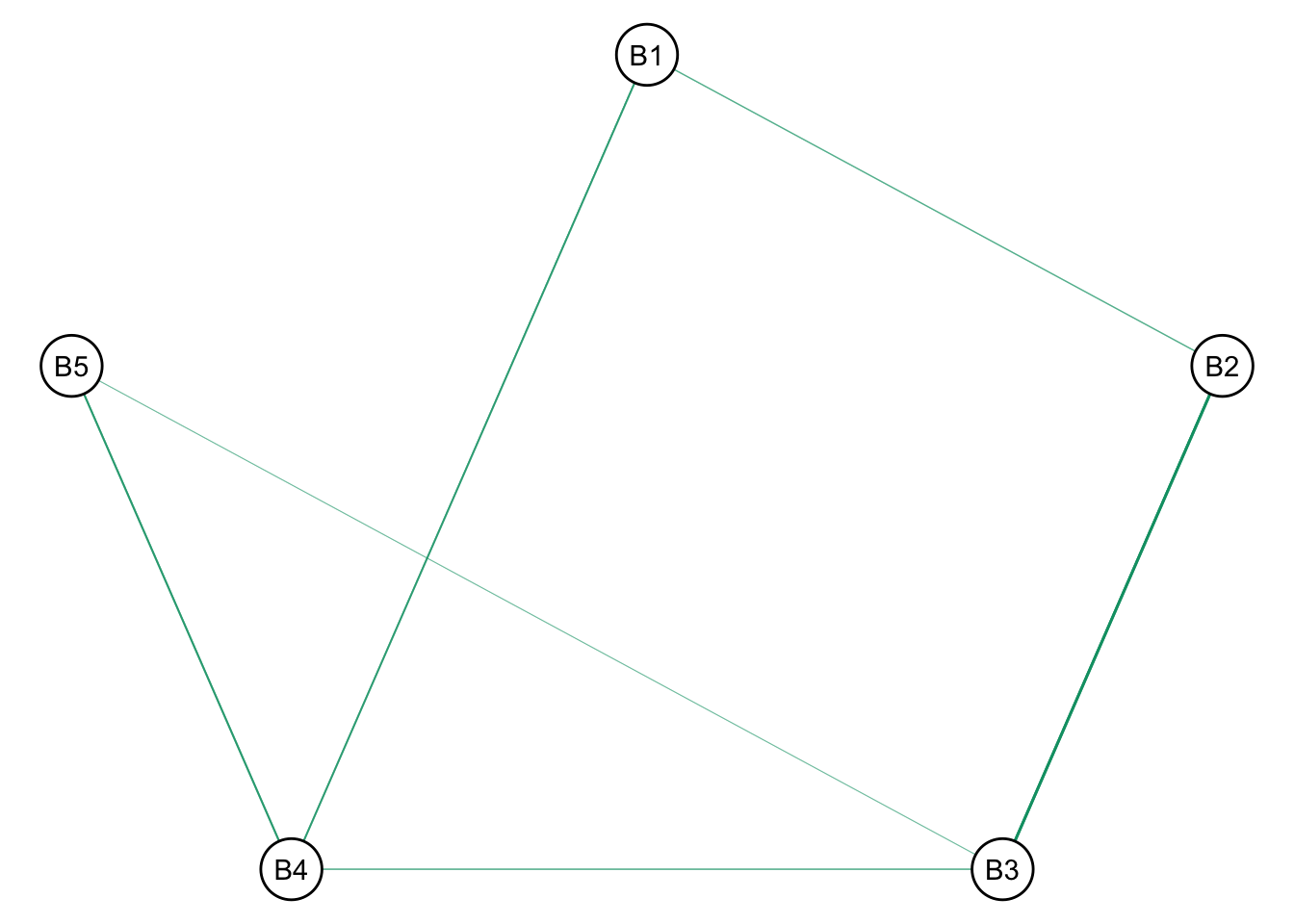
fit_reg <- BGGM::select(fit, alternative ="greater")plot(fit_reg)
$plt
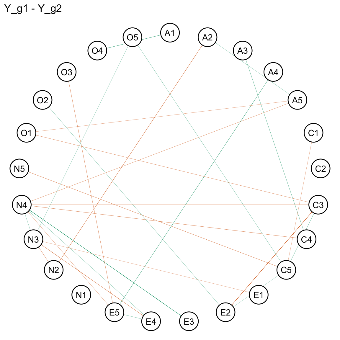
Hypothesis testing
Using BGGM, we can perform hypothesis testing like whether edge A is more strong than edge B, whether edge A is “significant” higher or smaller than 0, whether group A and group B have differences in partial correlations.
Testing Edge A vs. Edge B
Click to see the code
# example hypotheseshyp1 <-c("B2--B3 > B1--B4 > 0") # hypothesis 1hyp2 <-c("B1--B5 > B2--B5 > 0") # hypothesis 2hyp3 <-c("B2--B4 < 0") # hypothesis 3hyp4 <-c("B1--B3 < 0") # hypothesis 4## Posterior hypothesis probabilities.extract_php <-function(Y = Y, hypothesis = hyp, type ='ordinal') { x <-confirm(Y = Y, hypothesis = hypothesis, type = type) x_info <- x$info PHP_confirmatory <-as.matrix(x_info$PHP_confirmatory)rownames(PHP_confirmatory) <-c(x$hypothesis, "complement") PHP_confirmatory}extract_php(Y = Y, hypothesis = hyp1, type ='ordinal')
                     [,1]
B2--B3 > B1--B4 > 0 0.989
complement          0.011
Click to see the code
extract_php(Y = Y, hypothesis = hyp2, type ='ordinal')
                     [,1]
B1--B5 > B2--B5 > 0 0.866
complement          0.134
Click to see the code
extract_php(Y = Y, hypothesis = hyp3, type ='ordinal')
            [,1]
B2--B4 < 0 0.708
complement 0.292
Click to see the code
extract_php(Y = Y, hypothesis = hyp4, type ='ordinal')
            [,1]
B1--B3 < 0 0.253
complement 0.747
There are four hypothesis tested here:
The first expresses that the relation B2--B3 is larger than B1--B4 . In other words, that the partial correlation is larger for B2--B3. The p(H1|data) = 0.991 means the posterior hypothesis probability (PHP) is 0.991 which provides evidence for the hypothesis: the partial correlation for B2-B3 is larger;
The second expresses that the relation B1--B5 is larger than B2--B5 . The results of PHP suggests the hypothesis can be accepted;
The third expresses that the relation B2--B4 is larger than 0 . The results of PHP suggests the hypothesis can be accepted;
The fourth expresses that the relation B1--B3 is lower than 0 . The results of PHP suggests the hypothesis should be rejected given p(H1)<p(complement);
---title: 'How to use BGGM to Estimate Bayesian Gaussian Graphical Models'author: 'Jihong Zhang'subtitle: 'Bayesian version of GGM allows multiple Bayesian techniques to be used in psychological network.'date: 'Mar 5 2024'categories: - R - Bayesian - Tutorial - Network Analysisexecute: eval: true echo: true warning: falseformat: html: code-fold: true code-summary: 'Click to see the code'---> This is a quick note illustrate some importance functions of `BGGM` and illustrate them using one or more example(s).## Overview1. The [Github page](https://github.com/donaldRwilliams/BGGM) showcases some publications regarding algorithms of `GGGM`2. [Donny Williams's website](https://donaldrwilliams.github.io/BGGM/) has more examples## Illustrative Example 1```{r}pcor_to_df <-function(x, names =paste0("B", 1:5)) {colnames(x) =rownames(x) = names x_upper <- x x_upper[lower.tri(x_upper)] <-0as.data.frame(x_upper) |>rownames_to_column('Start') |>pivot_longer(-Start, names_to ='End', values_to ='Mean') |>filter(Mean !=0) |>mutate(Label =paste0(Start,'-', End)) }```A dataset containing items that measure Post-traumatic stress disorder symptoms (Armour et al. 2017). There are 20 variables (*p*) and 221 observations (*n*).### Estimation of Partial Correlation MatrixThe GGM can be estimated using `estimate` function with some important arguments:- `type`: could be `continuous`, `binary`, `ordinal`, or `mixed`- `iter`: Number of iterations (posterior samples; defaults to 5000).- `prior_sd`: Scale of the prior distribution, approximately the standard deviation of a beta distribution (defaults to 0.50).```{r}#| message: falselibrary(BGGM)library(tidyverse) # for ggplot2 and dplyrlibrary(psychonetrics) # the frequentist way for GGM# dataY <- ptsd[, 1:5] +1# add + 1 to make sure the ordinal variable start from '1'# ordinal modelfit <-estimate(Y, type ='ordinal', analytic =FALSE)fit_cont <-estimate(Y, type ='continuous', analytic =FALSE)#summary(fit)pcor_mat(fit)```Let's compare the partial correlation estimates to `psychonetrics````{r}#| warning: falsemod_saturated_ord <-ggm(Y, ordered =TRUE)mod_saturated_cont <-ggm(Y)getmatrix(mod_saturated_ord, 'omega')``````{r}#| fig-height: 8freqEst <-pcor_to_df(getmatrix(mod_saturated_ord, 'omega')) freqEst_cont <-pcor_to_df(getmatrix(mod_saturated_cont, 'omega')) # transform partial corr. mat. of BGGM into df.BayesEst <-pcor_to_df(pcor_mat(fit))BayesEst_cont <-pcor_to_df(pcor_mat(fit_cont)) combEst <-rbind( freqEst |>mutate(Type ='psychonetrics_ord'), BayesEst |>mutate(Type ='BGGM_ord'), freqEst_cont |>mutate(Type ='psychonetrics_cont'), BayesEst_cont |>mutate(Type ='BGGM_cont')) |>mutate(Type =factor(Type, levels =c("psychonetrics_ord", "BGGM_ord", "psychonetrics_cont","BGGM_cont")))ggplot(combEst) +geom_col(aes(x =fct_rev(Label), y = Mean, fill = Type, col = Type), position =position_dodge()) +geom_text(aes(x =fct_rev(Label), y =ifelse(Mean>0, Mean+.03, Mean-.03), label =round(Mean, 3), group = Type), position =position_dodge(width = .9)) +labs(x ='') +coord_flip() +theme_classic()```We can find that:1. Partial correlations with **ordinal** responses estimated by `psychonetric` **do not align well** with partial correlations with **ordinal** responses estimated by `BGGM`2. Partial correlations with **continuous** responses estimated by `psychonetric` **align well with** partial correlations with **continuous** responses estimated by `BGGM`3. Violating the continuous assumption of items responses usually underestimate the partial correlations (see `BGGM_cont` vs. `BGGM_ord`)### RegularizationIt is easy to conduct regularization using `Graph Selection` using hypothesis testing```{r}fit_reg <- BGGM::select(fit, alternative ="greater")plot(fit_reg)```### Hypothesis testingUsing `BGGM`, we can perform hypothesis testing like whether edge A is more strong than edge B, whether edge A is "significant" higher or smaller than 0, whether group A and group B have differences in partial correlations.#### Testing Edge A vs. Edge B```{r}# example hypotheseshyp1 <-c("B2--B3 > B1--B4 > 0") # hypothesis 1hyp2 <-c("B1--B5 > B2--B5 > 0") # hypothesis 2hyp3 <-c("B2--B4 < 0") # hypothesis 3hyp4 <-c("B1--B3 < 0") # hypothesis 4## Posterior hypothesis probabilities.extract_php <-function(Y = Y, hypothesis = hyp, type ='ordinal') { x <-confirm(Y = Y, hypothesis = hypothesis, type = type) x_info <- x$info PHP_confirmatory <-as.matrix(x_info$PHP_confirmatory)rownames(PHP_confirmatory) <-c(x$hypothesis, "complement") PHP_confirmatory}extract_php(Y = Y, hypothesis = hyp1, type ='ordinal')extract_php(Y = Y, hypothesis = hyp2, type ='ordinal')extract_php(Y = Y, hypothesis = hyp3, type ='ordinal')extract_php(Y = Y, hypothesis = hyp4, type ='ordinal')```There are four hypothesis tested here:1. The first expresses that the relation `B2--B3` is larger than `B1--B4` . In other words, that the partial correlation is larger for `B2--B3`. The `p(H1|data) = 0.991` means the posterior hypothesis probability (PHP) is `0.991` which provides evidence for the hypothesis: the partial correlation for `B2-B3` is larger;2. The second expresses that the relation `B1--B5` is larger than `B2--B5` . The results of PHP suggests the hypothesis can be accepted;3. The third expresses that the relation `B2--B4` is larger than 0 . The results of PHP suggests the hypothesis can be accepted;4. The fourth expresses that the relation `B1--B3` is lower than 0 . The results of PHP suggests the hypothesis should be rejected given $p(H_1) < p(complement)$;### Group Comparison```{r}#| cache: true# dataY <- bfi# malesYmales <-subset(Y, gender ==1, select =-c(gender, education))# femalesYfemales <-subset(Y, gender ==2, select =-c(gender, education))# model fitfit <-ggm_compare_estimate(Ymales, Yfemales)# plot summarysummary(fit)```The regularized group difference network plot can be visualized as:```{r}#| fig-width: 6#| fig-height: 6plot(BGGM::select(fit))```