library(tidyverse)
# or
library(lubridate)Class Outline
- Talk about the date-time variables
- Locales related to timezone
Introduction to Date-Time Parsing
Importance of Date-Time Data
- Dates and times are critical for tracking temporal data in analysis.
- Proper handling ensures accurate filtering, summarization, and visualization.
- Base R provides the
DateandPOSIXcttypes to manage date-time information.tidyverseprovides more types
Tip
You should always use the simplest possible data type that works for your needs. That means if you can use a date instead of a date-time, you should. Date-times are substantially more complicated because of the need to handle time zones, which we’ll come back to at the end of the chapter.
Using lubridate for Date-Time Parsing
Loading the Package
Create date/time variable
- Three types of date/time data that refer to an instant in time:
- A
date. - A
timewithin a day. - A
date-timeis a date plus a time: it uniquely identifies an instant in time (typically to the nearest second).- Tibbles prints this as
. Base R calls these POSIXct, but that doesn’t exactly trip off the tongue.
- Tibbles prints this as
- A
- To get the current date or date-time you can use
today()ornow():
today()[1] "2025-03-18"now()[1] "2025-03-18 11:03:39 CDT"Import
- If your CSV contains an ISO8601
dateordate-time, you don’t need to do anything;readr::read_csv()will automatically recognize it:
csv <- "
  date, datetime
  2022-01-02,2022-01-02 05:12
"
read_csv(csv)
# A tibble: 1 × 2
date datetime
<date> <dttm>
1 2022-01-02 2022-01-02 05:12:00
Tip
The date format follows ISO8601. If you haven’t heard of ISO8601 before, it’s an international standard for writing dates where the components of a date are organized from biggest to smallest separated by -. For example, in ISO8601 May 3 2022 is 2022-05-03.
If you date variable does not follow ISO8601…
For other date-time formats, you’ll need to use
col_types=pluscol_date()orcol_datetime()along with a date-time format.col_date()in readr package can uses a format specification- In which, data components are specified with “%” following by a letter
- For example, “%m” matches a 2-digit month; “%d” matches 2-digit day; “%y” matches 2-digit yaer: 00-69 -> 2000-2069
csv <- "
  ID,birthdate, datatime
  1,01/02/15, 2024.01.02
  2,02/03/15, 2024.01.03
"

read_csv(csv, col_types = cols(birthdate = col_date(format = "%m/%d/%y")))
# A tibble: 2 × 3
ID birthdate datatime
<dbl> <date> <chr>
1 1 2015-01-02 2024.01.02
2 2 2015-02-03 2024.01.03read_csv(csv, col_types = cols(birthdate = col_date(format = "%d/%m/%y")))# A tibble: 2 × 3
ID birthdate datatime
<dbl> <date> <chr>
1 1 2015-02-01 2024.01.02
2 2 2015-03-02 2024.01.03read_csv(csv, col_types = cols(birthdate = col_date(format = "%y/%m/%d")))# A tibble: 2 × 3
ID birthdate datatime
<dbl> <date> <chr>
1 1 2001-02-15 2024.01.02
2 2 2002-03-15 2024.01.03- Exercise: Try read in the data and convert the datatime into
dateobject
Date formats can be understood by readr
| Type | Code | Meaning | Example |
|---|---|---|---|
| Year | %Y |
4 digit year | 2021 |
%y |
2 digit year | 21 | |
| Month | %m |
Number | 2 |
%b |
Abbreviated name | Feb | |
%B |
Full name | February | |
| Day | %d |
One or two digits | 2 |
%e |
Two digits | 02 | |
| Time | %H |
24-hour hour | 13 |
%I |
12-hour hour | 1 | |
%p |
AM/PM | pm | |
%M |
Minutes | 35 | |
%S |
Seconds | 45 | |
%OS |
Seconds with decimal component | 45.35 | |
%Z |
Time zone name | America/Chicago | |
%z |
Offset from UTC | +0800 | |
| Other | %. |
Skip one non-digit | : |
%* |
Skip any number of non-digits |
The Date Type in base R
- Dates are stored as the number of days since January 1, 1970 (epoch reference).
as.Date("1970-01-01")[1] "1970-01-01"format(as.Date("1970-01-01"), format = "%Y/%m/%d")[1] "1970/01/01"- Convert character strings into
Dateformat:
as.Date("2025-02-13") # Convert string to Date type[1] "2025-02-13"- You can have access to the system date:
Sys.Date()[1] "2025-03-18"Parsing Date From String
lubridateprovides functions to interpret and standardize date formats.Parse dates with year, month, and day components
## heterogeneous formats in a single vector:
x <- c("2009-01-01", "09/01/02", "2009.Jan.2", "090102")
ymd(x)  # Interprets different formats correctly
[1] "2009-01-01" "2009-01-02" "2009-01-02" "2009-01-02"Handling Different Date Orders
Formats can be ambiguous,
lubridatehelps with appropriate parsing:- Once parsed, the object type will be converted to
Date
- Once parsed, the object type will be converted to
x <- "09/01/02"
ymd(x)  # Assumes year-month-day
[1] "2009-01-02"mdy(x) # Assumes month-day-year[1] "2002-09-01"dmy(x) # Assumes day-month-year[1] "2002-01-09"class(dmy(x))[1] "Date"Handling Date-Time with POSIXct
- Previous
Datetype variables contain year-month-day information - The
POSIXctclass stores timestamps as seconds since epoch. - Use
ymd_hms()to parse full date-time values:- Parse date-times with year, month, and day, hour, minute, and second components.
datetime_str <- "2025-02-12 14:30:00"
datetime <- ymd_hms(datetime_str)
print(datetime)
[1] "2025-02-12 14:30:00 UTC"- In
lubridate, there are various type of parsing functions that can parse the character based on the sequence of your date string
ymd_hms("2024-07-13 14:45:00")[1] "2024-07-13 14:45:00 UTC"ymd_hm("2024-07-13 14:45")[1] "2024-07-13 14:45:00 UTC"mdy_hm("07-13-2024 14:45")[1] "2024-07-13 14:45:00 UTC"mdy_hm("07.13.2024 14:45")[1] "2024-07-13 14:45:00 UTC"Example: Combine Multiple columns of date components into one date-time
- Instead of a single string, sometimes you’ll have the individual components of the date-time spread across multiple columns.
library(nycflights13)
flights_datetime <- flights |>
  select(year, month, day, hour, minute)
flights_datetime
# A tibble: 336,776 × 5
year month day hour minute
<int> <int> <int> <dbl> <dbl>
1 2013 1 1 5 15
2 2013 1 1 5 29
3 2013 1 1 5 40
4 2013 1 1 5 45
5 2013 1 1 6 0
6 2013 1 1 5 58
7 2013 1 1 6 0
8 2013 1 1 6 0
9 2013 1 1 6 0
10 2013 1 1 6 0
# ℹ 336,766 more rows- To create a date/time from this sort of input, use
make_date()for dates, ormake_datetime()for date-times:
flights_datetime |>
  mutate(departure_time = make_datetime(year, month, day, hour, minute),
         departure_date = make_date(year, month, day))
# A tibble: 336,776 × 7
year month day hour minute departure_time departure_date
<int> <int> <int> <dbl> <dbl> <dttm> <date>
1 2013 1 1 5 15 2013-01-01 05:15:00 2013-01-01
2 2013 1 1 5 29 2013-01-01 05:29:00 2013-01-01
3 2013 1 1 5 40 2013-01-01 05:40:00 2013-01-01
4 2013 1 1 5 45 2013-01-01 05:45:00 2013-01-01
5 2013 1 1 6 0 2013-01-01 06:00:00 2013-01-01
6 2013 1 1 5 58 2013-01-01 05:58:00 2013-01-01
7 2013 1 1 6 0 2013-01-01 06:00:00 2013-01-01
8 2013 1 1 6 0 2013-01-01 06:00:00 2013-01-01
9 2013 1 1 6 0 2013-01-01 06:00:00 2013-01-01
10 2013 1 1 6 0 2013-01-01 06:00:00 2013-01-01
# ℹ 336,766 more rowsCalculate departure time and arrival time
- In
flights,dep_timeandarr_timerepresents the time with the formatHHMMorHMM.- The first two digits contains hours; The second two digits contains minuts
dep_time %/% 100will be hoursdep_time %% 100will be minutes
flights |>
  select(dep_time) |>
  mutate(
    hours = dep_time %/% 100,
    minutes = dep_time %% 100,
  )
# A tibble: 336,776 × 3
dep_time hours minutes
<int> <dbl> <dbl>
1 517 5 17
2 533 5 33
3 542 5 42
4 544 5 44
5 554 5 54
6 554 5 54
7 555 5 55
8 557 5 57
9 557 5 57
10 558 5 58
# ℹ 336,766 more rowsCreate departure time
## create a self-made function that can read in HMM time format
make_datetime_100 <- function(year, month, day, time) {
  make_datetime(year, month, day, time %/% 100, time %% 100)
}

flights_dt <- flights |>
  filter(!is.na(dep_time), !is.na(arr_time)) |> # remove missing date
  mutate(
    dep_time = make_datetime_100(year, month, day, dep_time),
    sched_dep_time = make_datetime_100(year, month, day, sched_dep_time),
  ) |>
  select(origin, dest, dep_time, sched_dep_time)

flights_dt
# A tibble: 328,063 × 4
origin dest dep_time sched_dep_time
<chr> <chr> <dttm> <dttm>
1 EWR IAH 2013-01-01 05:17:00 2013-01-01 05:15:00
2 LGA IAH 2013-01-01 05:33:00 2013-01-01 05:29:00
3 JFK MIA 2013-01-01 05:42:00 2013-01-01 05:40:00
4 JFK BQN 2013-01-01 05:44:00 2013-01-01 05:45:00
5 LGA ATL 2013-01-01 05:54:00 2013-01-01 06:00:00
6 EWR ORD 2013-01-01 05:54:00 2013-01-01 05:58:00
7 EWR FLL 2013-01-01 05:55:00 2013-01-01 06:00:00
8 LGA IAD 2013-01-01 05:57:00 2013-01-01 06:00:00
9 JFK MCO 2013-01-01 05:57:00 2013-01-01 06:00:00
10 LGA ORD 2013-01-01 05:58:00 2013-01-01 06:00:00
# ℹ 328,053 more rowsVisualize distribution of departure time
- With this data, we can visualize the distribution of departure times on January 02, 2013
- use
%within% interval(start, end)to select a interval of two timestaps
- use
flights_dt |>
  filter(dep_time %within% interval("2013-01-03 00:00:00",
                                    "2013-01-04 00:00:00")) |>
  ggplot() +
  geom_histogram(aes(x = dep_time), fill = "skyblue", binwidth = 1800, alpha = .8)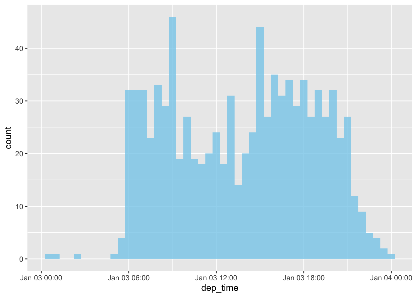
Get date/times as numeric offsets
- Sometimes you’ll get date/times as numeric offsets from the “Unix Epoch”, 1970-01-01. If the offset is in seconds, use as_datetime(); if it’s in days, use as_date().
as_datetime(60 * 60 * 10) # offset in seconds[1] "1970-01-01 10:00:00 UTC"as_date(365 * 10 + 2) # offset in days[1] "1980-01-01"Extracting Components From Date-Time
- Once parsed, individual components like year, month, or day information can be extracted for further analysis:
dates <- as.Date(c("2016-05-31 12:34:56",
                   "2016-08-08 12:34:56",
                   "2016-09-19 12:34:56"))

year(dates)  # Extract year
[1] 2016 2016 2016month(dates) # Extract month[1] 5 8 9day(dates) # Extract day[1] 31 8 19yday(dates) # day of the year[1] 152 221 263mday(dates) # day of the month[1] 31 8 19wday(dates) # day of the week[1] 3 2 2- For
month()andwday()you can set label = TRUE to return the abbreviated name of the month or day of the week
month(dates, label = TRUE) # day of the month[1] May Aug Sep
12 Levels: Jan < Feb < Mar < Apr < May < Jun < Jul < Aug < Sep < ... < Decwday(dates, label = TRUE) # day of the week[1] Tue Mon Mon
Levels: Sun < Mon < Tue < Wed < Thu < Fri < SatModify Components From Date-Time
- You can use
year() <-,month() <-, andhour() <-to modify year, month, and hours of original date-time object
(datetime <- ymd_hms("2026-07-08 12:34:56"))[1] "2026-07-08 12:34:56 UTC"year(datetime) <- 2030
datetime[1] "2030-07-08 12:34:56 UTC"month(datetime) <- 01
datetime[1] "2030-01-08 12:34:56 UTC"hour(datetime) <- hour(datetime) + 1
datetime[1] "2030-01-08 13:34:56 UTC"Rounding the Date
floor_date(),round_date(), andceiling_date()are useful to adjusting our dates. Each function takes a vector of dates to adjust and then the name of the unit to round down (floor), round up (ceiling), or round to.
dates <- as.Date(c("2016-05-31 12:34:56",
                   "2016-08-08 12:34:56",
                   "2016-09-19 12:34:56"))
floor_date(dates, unit = "week") # Sunday of the week
[1] "2016-05-29" "2016-08-07" "2016-09-18"wday(dates)[1] 3 2 2floor_date(dates, unit = "week") |> wday()[1] 1 1 1ceiling_date(dates, unit = "week") # Saturday of the week[1] "2016-06-05" "2016-08-14" "2016-09-25"Example: distribution of number of flights by week days
Distribution of number of flights by week
flights_dt |>
  count(week = floor_date(dep_time, "week")) |>
  ggplot(aes(x = week, y = n)) +
  geom_line() +
  geom_point()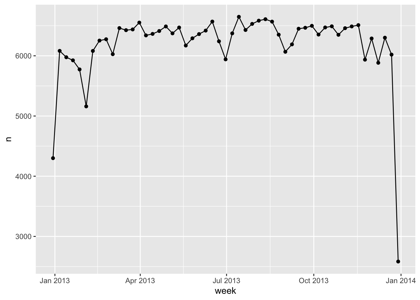
Time Spans
Three important classes that represent time spans:
- Durations, which represent an exact number of seconds.
- Periods, which represent human units like weeks and months.
- Intervals, which represent a starting and ending point.
In R, when you subtract two dates, you get a
difftimeobject:
# How old is Hadley?
h_age <- today() - ymd("1979-10-14")
h_age
Time difference of 16592 daysclass(h_age)[1] "difftime"
Tip
A difftime class object records a time span of seconds, minutes, hours, days, or weeks.
Duration: fixed time length
lubridatepackage provides an alternative which always uses seconds: the duration.
h_duration <- as.duration(h_age)

dseconds(h_duration)
[1] "1433548800s (~45.43 years)"dminutes(1) # one minute difference[1] "60s (~1 minutes)"dhours(2) # 2 hours differences[1] "7200s (~2 hours)"ddays(4) # 4 days differences[1] "345600s (~4 days)"dweeks(2) # 2 weeks difference[1] "1209600s (~2 weeks)"dyears(1.5) # one and half year difference[1] "47336400s (~1.5 years)"- Calculation use old_date + duration = new_date
- Next lecture’s date
ymd("2025-02-20") + dweeks(1)[1] "2025-02-27"However, because durations represent an exact number of seconds, sometimes you might get an unexpected result:
- March 8 only has 23 hours because it’s when DST starts, so if we add a full days worth of seconds we end up with a different time.
one_am <- ymd_hms("2026-03-08 01:00:00", tz = "America/New_York")

one_am
[1] "2026-03-08 01:00:00 EST"one_am + ddays(1) # Time changes because of the changes from EST (Eastern Standard Time) to EDT (Eastern Daylight Time)[1] "2026-03-09 02:00:00 EDT"Period: “human” times
Periods are time spans but don’t have a fixed length in seconds, instead they work with “human” times, like days and months.
- That allows them to work in a more intuitive way:
one_am[1] "2026-03-08 01:00:00 EST"one_am + days(1)[1] "2026-03-09 01:00:00 EDT"Locales and Time zones
Time Zones
- In R, the time zone is an attribute of the
date-timethat only controls printing. For example, these three objects represent the same instant in time:
x1 <- ymd_hms("2024-06-01 12:00:00", tz = "America/New_York")
x1
[1] "2024-06-01 12:00:00 EDT"x2 <- ymd_hms("2024-06-01 18:00:00", tz = "Europe/Copenhagen")
x2[1] "2024-06-01 18:00:00 CEST"x3 <- ymd_hms("2024-06-02 04:00:00", tz = "Pacific/Auckland")
x3[1] "2024-06-02 04:00:00 NZST"x1 - x2Time difference of 0 secsx1 - x3Time difference of 0 secs- You can also use
difftimeto calculate time different across different time zones
dublin_time <- ymd_hm("2001-10-10 20:10", tz = "Europe/Dublin")
hk_time <- ymd_hm("2001-10-10 20:10", tz = "Asia/Hong_Kong" )
time_diff <- difftime(dublin_time, hk_time, units = "hours")
days(time_diff)
[1] "7d 0H 0M 0S"Checking Timezones
You can see a complete list of time zones with OlsonNames().
Sys.timezone(location = TRUE) ## check your time zone in your computer system[1] "America/Chicago"head(OlsonNames())[1] "Africa/Abidjan" "Africa/Accra" "Africa/Addis_Ababa"
[4] "Africa/Algiers" "Africa/Asmara" "Africa/Asmera" Change time zone
- You can display date-time in another time zone:
x <- ymd_hms("2009-08-07 00:00:01", tz = "America/New_York")
with_tz(x, "Asia/Hong_Kong")
[1] "2009-08-07 12:00:01 HKT"x4 <- c(x1, x2, x3)
x4[1] "2024-06-01 12:00:00 EDT" "2024-06-01 12:00:00 EDT"
[3] "2024-06-01 12:00:00 EDT"with_tz(x4, tzone = "Australia/Lord_Howe")[1] "2024-06-02 02:30:00 +1030" "2024-06-02 02:30:00 +1030"
[3] "2024-06-02 02:30:00 +1030"Checking and Setting Locales
What are Locales?
The settings related to the language and the regions in which computer program executes.
Locales define how dates, times, numbers, and character encodings are interpreted.
Key aspects include:
- Date and time formats
- Time zones
- Character encoding
- Decimal and grouping symbols
Sys.getlocale()[1] "en_US.UTF-8/en_US.UTF-8/en_US.UTF-8/C/en_US.UTF-8/en_US.UTF-8"Sys.setlocale("LC_ALL", "en_US.UTF-8")[1] "en_US.UTF-8/en_US.UTF-8/en_US.UTF-8/C/en_US.UTF-8/en_US.UTF-8"LC_TIME: Controls date-time formatting.LC_NUMERIC: Determines the decimal and grouping symbols.
Handling Different Locales
- Using
readr::locale() - The
readrpackage allows setting locales while reading data.
library(readr)
locale()
<locale>
Numbers: 123,456.78
Formats: %AD / %AT
Timezone: UTC
Encoding: UTF-8
<date_names>
Days: Sunday (Sun), Monday (Mon), Tuesday (Tue), Wednesday (Wed), Thursday
(Thu), Friday (Fri), Saturday (Sat)
Months: January (Jan), February (Feb), March (Mar), April (Apr), May (May),
June (Jun), July (Jul), August (Aug), September (Sep), October
(Oct), November (Nov), December (Dec)
AM/PM: AM/PM- Specifying a locale allows you to parse dates in other languages:
parse_date("1 janvier 2015", "%d %B %Y", locale = locale("fr"))[1] "2015-01-01"parse_date("14 oct. 1979", "%d %b %Y", locale = locale("fr"))[1] "1979-10-14"parse_date("1994年10月01日", "%Y年%m月%d日", locale = locale("zh"))[1] "1994-10-01"See vignette("locales") for more details
Summary
lubridatesimplifies parsing and manipulating date-time data.- Converting text-based dates into structured
DateandPOSIXctformats enables powerful analysis. - Handling time zones correctly ensures accurate comparisons across regions.