Lecture 09: Introduction to Two-Way ANOVA

Overview of Lecture 09 & Lecture 10

1. The rest of the semester
2. Advantages of Factorial Design
3. Two-way ANOVA:
   • Steps for conducting two-way ANOVA
   • Hypothesis testing
   • Assumptions of two-way ANOVA
   • Visualization
   • Difference between one-way and two-way ANOVA

1 Previous lectures

Note

• In experimental design, when we are interested in comparing the means of dependent variable among several groups:

  • z-test
    1. A group vs. the population
  • t-test
    1. One group vs. another group
  • One-way ANOVA
    1. More than two groups

NoteExamples of z-test, t-test, and one-way ANOVA

Z-test: A school claims that the average score of students on a national exam is 75. A sample of 40 students has a mean score of 78. A z-test compares the sample mean to the population mean of 75.

t-test: A researcher compares test scores between two groups of students: one using online learning and the other using traditional classroom learning. A t-test determines whether there is a significant difference between the two groups’ scores.

One-way ANOVA: A scientist tests the effectiveness of three drug treatments on blood pressure reduction. Three groups of patients receive different treatments, and a one-way ANOVA assesses whether there are significant differences among the three groups.

2 Block Design: IV and Extraneous Factor

Important

1. When comparing the means of DV among several groups with more than two IVs, we can use :
   1. Blocking Design
      • Independent variable: the factor of the interest (→ the factor that we expect to have any meaningful impact on the dependent variable)
      • Extraneous factor → the factors that impacts on DV

Note

Independent Variable: In a study investigating the impact of different teaching methods (e.g., traditional, online, and blended) on student performance, the independent variable would be the type of teaching method, as it’s the factor being manipulated to assess its effect on student performance.

Extraneous Variable: In the same study, an extraneous variable could be the students’ prior knowledge or their baseline academic performance, as this could influence their learning outcomes but is not the main focus of the research. This variable might affect the dependent variable (student performance) but is not part of the experimental manipulation.

3 Block Design Review: IV and Extraneous Factor

Important

1. If an extraneous factor is expected to affect the IV as well, it is treated as a confounding factor
2. If an extraneous factor is not expected to affect the IV, it is treated as a nuisance factor
   1. If the nuisance variable is known and controllable, use blocking by including a blocking factor in the experiment.
   2. If the nuisance factor is known but uncontrollable, use ANCOVA to adjust for its effect.
   3. If nuisance factors are unknown and uncontrollable (sometimes called “lurking” variables; e.g., teachers’ personality/emotions), use randomization to balance their impact.

NoteExamples of Independent, Confounding Factor, and Nuisance Factor

1. Confounding Factor
   • A study examines the effect of a new medication (IV) on blood pressure (DV). Dietary habits influence both the medication adherence and blood pressure, making it a confounding factor.
2. Nuisance Factors
   • Known and Controllable (Blocking Factor)
     • A study on fertilizer effectiveness (IV) on crop yield (DV) includes different farms as a blocking factor to account for variations in soil quality.
       
   • Known but Uncontrollable (Covariate in ANCOVA)
     • A study on the effect of a math intervention (IV) on test scores (DV) includes students’ prior math knowledge as a covariate in ANCOVA.
       
   • Unknown and Uncontrollable (Lurking Variable, Balanced via Randomization)
     • A study on online learning effectiveness (IV) on student performance (DV) may have students’ intrinsic motivation as an unknown, uncontrollable nuisance factor. Randomization helps mitigate its influence.
       

4 Factorial Design: History, Popularity, and Blocking

NoteBrief History of Factorial Design

• Early experiments (18th–19th c.) often varied one factor at a time (OFAT), which missed interactions and was inefficient.
• R. A. Fisher (1920s–1930s) at Rothamsted formalized randomization, blocking, and factorial experiments, showing how to estimate main effects and interactions efficiently.
• Post–WWII developments (e.g., Box): response surface methods, 2^k and fractional factorials for industrial screening; widespread adoption across agriculture, engineering, pharma, psychology, and education.
• Modern practice: DOE software and mixed models generalize factorials to unbalanced, hierarchical, and repeated‑measures settings.

---

TipWhy Factorial Designs Are Popular

• Detect interactions: quantify whether the effect of one factor depends on another (moderation).
• Efficiency and power: estimate multiple effects in one study; including relevant factors reduces residual variance and increases power.
• External validity: mirrors real systems where multiple influences co-occur.
• Clearer inference: main effects estimated while controlling for other designed factors.
• Flexibility: extends to mixed/split‑plot/repeated‑measures and generalized linear models.

---

CautionFactorial vs. Block Designs (Different Purposes)

• Factorial design: manipulates two or more substantive factors of interest; estimates main effects and interactions.
• Blocking: groups units by known nuisance structure (fields, classrooms, batches) to reduce error variance; blocks are not the primary scientific factors.
• Often combined: factorial‑with‑blocking (e.g., randomized complete block with crossed treatment factors) or split‑plot factorials when randomization differs across factors.
• Popularity depends on field and goal: agriculture uses both extensively; industry favors factorials for screening plus blocking by shift/batch; social sciences use factorials for moderation and handle blocks via design or mixed models.

---

NoteQuick Guidance

• Use blocking when you can form homogeneous groups that differ from each other but are not of substantive interest.
• Use factorial design when you have ≥2 substantive factors and care about both separate effects and interactions.
• Use factorial‑with‑blocking when both conditions hold; consider split‑plot when application/randomization constraints differ across factors.

5 Types of Factorial Design

2. When we are interested in comparing the means of dependent variable among several groups with more than two independent variables:
3. Factorial Design
   • Independent or between-subject design
     • Each individual is in only 1 group or receives only 1 treatment
   • Dependent and/or repeated-measure design
     • Each individual is in each of the groups or receives each of the treatments
   • Mixed design (e.g., split-plot design, etc.)
     • For one IV, each individual is in 1 group or receives 1 treatment
     • For the other IV, each individual is in each of the groups or receives each of the treatments

---

TipExamples of multi-way ANOVA

• For 2 IVs, each person is in only one group = two-way independent ANOVA
• For 3 IVs, each person receives each treatment = three-way repeated-measures ANOVA
• For 2 IVs, each person receives one treatment for one IV and each treatment for the other IV = two-way mixed ANOVA

Note. “A (number of IVs)-way (type of design) ANOVA” → The label changes as the number of factors increases.

6 Difference of Factorial Design

Design Type	Key Feature	Example	Statistical Analysis
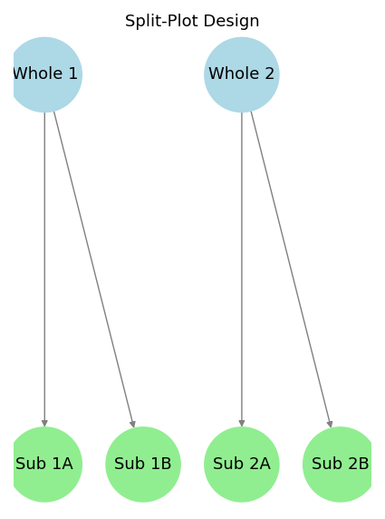
Split-Plot	Hierarchical treatment assignment (whole plots and subplots)	Agriculture: Irrigation (whole plot) & Fertilizer (subplot)	Mixed-effects model
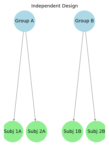
Independent	Each participant/unit is exposed to one condition only	Teaching Method 1 vs. Method 2	Independent t-test, ANOVA
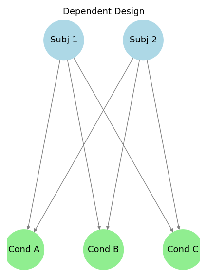
Dependent	Same participant/unit exposed to all conditions	Measuring reaction time with different caffeine levels	Repeated-measures ANOVA, mixed-effects model

7 Example of Factorial Design

Important

• Research Question: Is there an interaction between school type and tutoring program on academic achievement?
  • For this RQ, we might think that the effect of tutoring program depends on the type of school the students attend.
  • As shown below, there are three levels for the tutoring program (e.g., no tutor, once a week, and daily) and three levels for the school type (e.g., public, private-secular, and private-religious).
  • Then, we examine ALL combinations of the levels of these two IVs.

School\Program	No Tutor	Once Per Week	Daily
Public	Y11	Y12	Y13
Private-secular	Y21	Y22	Y23
Private-religious	Y31	Y32	Y33

• This would be a 3 x 3 design: two factors, one with 3 levels and one with 3 levels
  • 3 levels of tutoring program
  • 3 levels of school type
• Complete term: 3 x 3 two-way ANOVA or 3 x 3 independent factorial ANOVA

8 Example of Factorial Design

Caution

Question: What kind of design is used in the following research question?

• Does the effect of three different drug treatments (separate groups for Drug A, Drug B, Placebo) on self-reported positive mood depend on whether the participant received psychotherapy (treatment group) or not (control group)?
  1. One-way repeated-measure ANOVA
  2. 2 x 3 split-plot factorial ANOVA
  3. 2 x 3 independent factorial ANOVA
  4. 2 x 3 repeated-measure factorial ANOVA
• Answer: C
  • We have two IVs: drug treatment and therapy.
  • One factor, therapy, has two levels: treatment (therapy = yes), control (therapy = no).
  • The other factor, drug treatment, has three levels: Drug A, Drug B, and Placebo.
  • This design does not have within-subject (repeated-measures) components.
  • Generally, list the factor with fewer levels first.
  • So, this is an example of 2 x 3 independent factorial ANOVA.

9 Example of Factorial Design

Caution

Question: What kind of design is used in the following research question?

• Does the number of hours studied differ by university (UA, UAFS, UALR) and by semester (Fall, Spring, Summer) across academic cohorts (2012–2015)? A different sample of students was taken each semester.
  1. 3 x 3 x 4 independent factorial ANOVA
  2. 3 x 3 x 4 split-plot factorial ANOVA
  3. 3 x 4 independent factorial ANOVA
  4. 3 x 4 repeated-measure factorial ANOVA
• Answer: A
  • We have three IVs: school, semester, and cohort. School has three levels (UA, UAFS, UALR); semester has three levels (Fall, Spring, Summer); cohort has four levels (2012, 2013, 2014, 2015).
  • This design does not include within-subject (repeated-measures) components because a different sample of students was taken each semester.
  • Generally, the smaller number of levels comes the first.
  • So, this is an example of 3 x 3 x 4 independent factorial ANOVA.

10 Advantages of Factorial Design

• Factorial designs offer several advantages over a one-way ANOVA:
  1. It allows for greater generalizability of results
     • More realistic (external validity)
     • Example: Comparing a study with participants from multiple age groups (childhood and youth) versus a study including only youth
  2. It allows for investigation of interactions (answer more complicated RQs)
     • We can ask whether the effect of one variable depends on the level of another
     • Example: cancer trials; Does the effect of treatment method depend on cancer stage?
  3. It requires fewer participants than two one-way designs for the same level of statistical power.
     • Smaller error terms mean more statistical power.

---

10.1 Example: Cancer Trials

• Below is an R script demonstrating a factorial design for a cancer trial where the goal is to examine whether the effect of a treatment method depends on the stage of cancer (i.e., testing for an interaction effect).

Evaluating hidden code cell...

1

2

3

4

5

6

7

8

9

10

11

table(cancer_data$Treatment, cancer_data$Stage)

# Perform two-way ANOVA

anova_model <- aov(Survival ~ Treatment * Stage, data = 

cancer_data)

summary(anova_model)

# Interaction plot

interaction.plot(cancer_data$Stage, 

cancer_data$Treatment, cancer_data$Survival,

                 col = c("blue", "red"), lty = 1, pch = 

                 19, 

                 main = "Interaction Between Treatment 

                 and Cancer Stage",

                 xlab = "Cancer Stage", ylab = "Mean 

                 Survival Rate")

11 Interpretation of Results

NoteInterpretation of Results

• If the main effect of tutoring is significant, then grades differ across tutoring conditions, regardless of school type.

• If the main effect of school type is significant, then grades differ across school types, regardless of tutoring.

• If the interaction effect (Tutoring × School) is significant, then the impact of tutoring depends on school type, suggesting that different tutoring programs work better in different school settings.
  

12 Advantages of Factorial Design

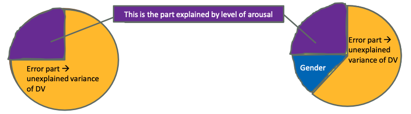
1. One advantage of factorial design is reducing error variance, which increases power to detect group differences.

ImportantExample: Effect of arousal on math performance

• Suppose we want to test the effect of arousal (e.g., anxiety) on math performance and suspect that gender is associated with performance.
  • Adding gender as an IV explains more variance and reduces error variance in the DV.
  • Note: We define error as anything not explained by the IVs.
    

13 Advantages of Factorial Design III

1. One key advantage of factorial design is that it allows us to consider more complicated scenarios by including multiple factors in a single experiment. This means we can analyze not only the main effects of each factor but also their interactions, providing deeper insights into real-world complexities.

NoteCancer Trial Example: Expanding the Factorial Design

• In the previous example, we considered a 2×2 factorial design with two factors:

  • Treatment Method (Standard vs. New)
  • Cancer Stage (Early vs. Advanced)

• However, real-world cancer treatments involve more than two factors. For instance, we might also want to consider:

  • Dosage Level (Low vs. High)
  • Patient Age Group (Young vs. Elderly)

• By extending the factorial design to a 2×2×2×2 factorial structure, we can investigate more complex research questions, such as:

  1. Does the effectiveness of a treatment vary not only by cancer stage but also by dosage level?
  2. Do younger and older patients respond differently to a specific combination of treatment and dosage?
  3. Is there a three-way interaction, where the best treatment strategy depends on a combination of treatment type, cancer stage, and dosage level?

---

13.1 Cancer Trial Example: Why Is This Important

ImportantWhy Is This Important?

• Better Understanding of Individual Differences:
  • A one-factor design (e.g., comparing only treatment types) would ignore how different patient groups respond differently to the same treatment.
  • By incorporating multiple factors, we can identify which subgroups benefit most from a specific intervention.
• More Realistic Clinical Applications:
  • In real-world medicine, treatment effectiveness depends on multiple interacting factors.
  • A factorial design helps us replicate complex clinical settings more accurately than a simple one-factor experiment.
• Efficient Use of Resources:
  • Instead of conducting multiple separate studies to test each factor independently, factorial design allows us to study all factors simultaneously in a single experiment.
  • This reduces costs and increases statistical power by leveraging shared data across conditions.

14 One-Way vs. Two-Way ANOVA

NoteKey Differences

• One-way ANOVA
  • Tests mean differences across levels of a single factor (one IV).
  • Provides one F-test for that factor’s main effect.
  • Cannot estimate interactions and ignores potential moderation by a second factor.
• Two-way ANOVA
  • Tests two main effects (Factor A and Factor B) and their interaction (A × B).
  • Estimates each main effect while controlling for the other factor.
  • Reveals whether the effect of one factor depends on the level of the other (interaction).

---

ImportantWhy Prefer Two-Way ANOVA (When Appropriate)

• Detect interactions
  • Real-world effects often depend on context; interactions identify when a treatment works better for some groups/conditions than others.
• Improve precision (reduce error variance)
  • Including a second relevant factor explains additional variance in the DV, increasing statistical power.
• Greater external validity
  • Modeling multiple factors better reflects applied settings where several influences co-occur.
• Efficiency
  • Studying two factors together can require fewer participants than two separate one-way studies for the same power.
• Clearer interpretation
  • Main effects are estimated while controlling for the other factor, yielding cleaner comparisons than multiple one-way ANOVAs.

15 Two-Way ANOVA vs. Mixed-Effects Model

NoteWhen to Prefer Mixed-Effects over Two-Way ANOVA

• Hierarchical or nested data
  • Examples: students within classrooms, patients within clinics, plots within fields, repeated observations within subjects.
  • Rationale: observations within the same group are correlated; random effects model this correlation and protect Type I error.
• Many groups you do not want as fixed effects
  • Examples: dozens of classrooms/teachers/batches.
  • Rationale: estimating many fixed levels is inefficient; random effects treat groups as a sample with partial pooling and population-level inference.
• Unbalanced or partially missing cells
  • Some groups lack certain factor combinations or have unequal n.
  • Mixed models accommodate this more flexibly than classical ANOVA.
• Repeated measures/longitudinal data
  • Use random intercepts/slopes to capture within-unit correlation and heterogeneity in trajectories.
• Heterogeneous variance/correlation structures
  • Mixed models allow residual variance/covariance structures beyond homoscedastic, independent errors.
• Generalization beyond observed levels
  • Inference about “classrooms in general,” not just the ones sampled.

---

TipTypical Modeling Setups

• Random intercepts: Score ~ Treatment + (1 | Classroom)
  • Captures classroom baseline differences.
• Random intercepts and slopes: Score ~ Treatment + (1 + Treatment | Classroom)
  • Allows treatment effects to vary across classrooms (cross-level interaction).
• Crossed random effects: Score ~ Treatment + (1 | Student) + (1 | Rater)
  • For designs with multiple random sources not nested within each other.
• Split-plot analogs: factors applied at different hierarchy levels
  • Mixed models mirror correct error terms via random effects.

---

CautionWhen Two-Way ANOVA Is Still Appropriate

• Factors are fully crossed, fixed, and of substantive interest.
• Design is (near) balanced with independent observations and homogeneous residual variances.
• No nesting or repeated measures; or blocking can be handled as a fixed factor with adequate replication.

NoteRule of Thumb

• If units are grouped within higher-level units or you want population-level inference across many groups, prefer mixed-effects.
• If you have few, specific groups of direct interest and assumptions hold, a fixed-effects two-way ANOVA can be sufficient.

16 Steps for conducting two-way ANOVA

• Similar to one-way ANOVA:
  1. Set the null hypothesis and the alternative hypothesis → Research question?
  2. Find the critical value of the test statistic (F-critical) based on alpha and df.
  3. Calculate the observed value of the test statistic (F-observed) based on the sample.
  4. Make the statistical conclusion → either reject or retain the null hypothesis
  5. State the research conclusion regarding the research question.

17 Hypothesis testing for two-way ANOVA (I)

• For two-way ANOVA, there are three distinct hypothesis tests:
  • Main effect of Factor A
  • Main effect of Factor B
  • Interaction of A and B

NoteDefinition

F-test

Three separate F-tests are conducted for each!

Main effect

Occurs when there is a difference between levels for one factor

Interaction

Occurs when the effect of one factor on the DV depends on the level of the other factor

Said another way, when the difference in one factor is moderated by the other

Said a third way, the difference between levels of one factor depends on the other factor

18 Hypothesis testing for two-way ANOVA (II)

ImportantExample

Background: A researcher investigates how study method (Factor A: Lecture vs. Interactive) and test format (Factor B: Multiple-choice vs. Open-ended) affect student performance (DV: test scores). Students are randomly assigned to one of the two study methods and then assessed on one of the two test formats.

• Main Effect of Study Method (Factor A):
  • H0: There is no difference in test scores between students who used the lecture method and those who used the interactive method.
  • H1: There is a difference in test scores between the two study methods.
• Main Effect of Test Format (Factor B):
  • H0: There is no difference in test scores between students taking a multiple-choice test and those taking an open-ended test.
  • H1: There is a difference in test scores between the two test formats.
• Interaction Effect (Study Method × Test Format):
  • H0: The effect of study method on test scores is the same across test formats.
  • H1: The effect of study method on test scores depends on the test format (i.e., there is an interaction).

19 Hypothesis testing for two-way ANOVA (III)

1. Hypothesis test for a main effect with more than two levels

   • Mean differences among levels of one factor:

     1. Differences are tested for statistical significance
     2. Each factor is evaluated independently of the other factor(s) in the study.

   • Factor A’s main effect: “Controlling for Factor B, are there differences in the DV across Factor A?”

     $H_0$: $\mu_{A_1}=\mu_{A_2}=\cdots=\mu_{A_k}$

     $H_1$: At least one $\mu_{A_i}$ differs from the others in Factor A

   • Factor B’s main effect: “Controlling for Factor A, are there differences in the DV across Factor B?”

     $H_0$: $\mu_{B_1}=\mu_{B_2}=\cdots=\mu_{B_k}$

     $H_1$: At least one $\mu_{B_i}$ differs from the others in Factor B

Caution

Question: What does “controlling” mean in “Controlling for Factor A, …”?

Answer: “Controlling” means accounting for Factor A’s effect when evaluating Factor B, thereby reducing unexplained (error) variance.

20 FAQ: Number of Factor Levels

NoteDoes the number of groups (levels) matter in two-way ANOVA?

• Definition: In two-way ANOVA, “groups” are the a × b cells formed by levels of Factor A (a levels) and Factor B (b levels).
• Validity: The ANOVA framework supports any a, b ≥ 2; having many levels (e.g., 10+) is not inherently a problem.

---

TipPractical Considerations with Many Levels

• Sample size per cell: Ensure adequate and preferably balanced n per cell; power for main effects and interactions depends on per‑cell n and total cells (a × b).
• Assumptions: Check residual normality and homogeneity of variances across cells; with many small‑n cells, violations are harder to detect and more influential.
• Multiple comparisons: Many levels imply many pairwise tests—use planned contrasts or adjust p‑values (e.g., Tukey, Holm).
• Model degrees of freedom: More levels increase df for main effects and interactions; plan total N accordingly to avoid low power.
• Empty/near‑empty cells: Sparse cells destabilize interaction estimates; redesign, combine levels (if justified), or increase n.

---

CautionAlternatives and Modeling Strategies

• Ordered factors (e.g., doses): Use polynomial trend contrasts rather than all pairwise comparisons.
• Many nuisance levels (e.g., classrooms, batches): Consider mixed‑effects models with the high‑level factor as random.
• Heteroscedasticity: Consider variance‑stabilizing transforms, Welch‑type methods, GLS, or robust ANOVA.

21 Hypothesis testing for two-way ANOVA (IV)

NoteExample: Tutoring Program and School Type on Grades

• IVs:
  1. Tutoring Programs: (1) No tutor; (2) Once a week; (3) Daily
  2. Types of schools: (1) Public (2) Private-secular (3) Private-religious
• Research purpose: Examine the effects of tutoring program (no tutor, once a week, daily) and school type (public, private-secular, private-religious) on students’ grades.
• Question: What are the null and alternative hypotheses for the main effects in this example?

  • Factor A’s main effect: “Controlling for school type, are there differences in students’ grades across the three tutoring programs?”

    $H_0$: $\mu_{\mathrm{no\ tutor}}=\mu_{\mathrm{once\ a\ week}}=\mu_{\mathrm{daily}}$

  • Factor B’s main effect: “Controlling for tutoring program, are there differences in students’ grades across the three school types?”

    $H_0$: $\mu_{\mathrm{public}}=\mu_{\mathrm{private-religious}}=\mu_{\mathrm{private-secular}}$

22 Visualization of Two-Way ANOVA (No Interaction)

• The main-effects-only, no-interaction model

$$\mathrm{Grade} = \beta_0 + \beta_1 \mathrm{Tutoring_{Once}} + \beta_2 \mathrm{Tutoring_{Daily}} \\ + \beta_3 \mathrm{SchoolType_{PvtS}} + \beta_4 \mathrm{SchoolType_{PvtR}}$$

Evaluating hidden cell 1 out of 2

• Main effect of Tutoring Programs
  • Collapsing across School Type
  • Ignoring the difference levels of School Type
  • Averaging DV regarding Tutoring Programs across the levels of School Type
• Main effect of School Type
  • Collapsing across Tutoring Program
  • Ignoring the difference levels of Tutoring Program
  • Averaging DV regarding School Type across the levels of Tutoring Programs

---

R plot

# Compute mean and standard error for each tutoring group
tutoring_summary <- data |>
  group_by(Tutoring) |>
  summarise(
    Mean_Grade_byTutor = mean(Grades),
    School = factor(c("Public","Private-Secular", "Private-Religious"), 
                    levels = c("Public","Private-Secular", "Private-Religious"))
  ) 

school_summary <- data |>
  group_by(School) |>
  summarise(
    Mean_Grade_bySchool = mean(Grades)
  ) 

total_summary <- tutoring_summary |> 
  left_join(school_summary, by = "School")

# Plot main effect of tutoring
ggplot(total_summary, aes(x = School)) +
  geom_point(aes(y = Mean_Grade_byTutor, color = Tutoring), size = 5) +
  geom_hline(aes(yintercept = Mean_Grade_byTutor, color = Tutoring), linewidth = 1.3) +
  scale_y_continuous(limits = c(70, 90), breaks = seq(70, 90, 5)) +
  labs(title = "Main Effect of Tutoring on Student Grades",
       x = "School Types",
       y = "Mean Grade") +
  theme_minimal() +
  theme(legend.position = "none")  # Remove legend for cleaner visualization

Summary statistics

distinct(tutoring_summary[, c("Tutoring", "Mean_Grade_byTutor")])

# A tibble: 3 × 2
# Groups:   Tutoring [3]
  Tutoring    Mean_Grade_byTutor
  <fct>                    <dbl>
1 No Tutor                  76.6
2 Once a Week               81.1
3 Daily                     86.3

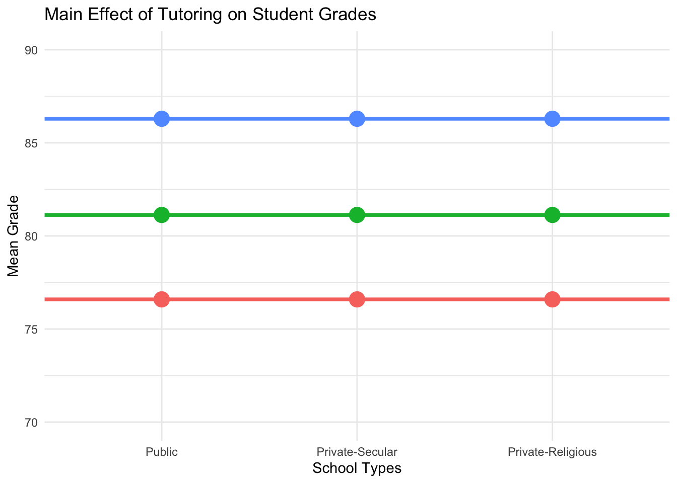
Interpretation of the plot

• The x-axis represents three school types.
• The y-axis represents the mean student grades for the different tutoring programs: No Tutor, Once a Week, and Daily.
• If the main effect of tutoring is significant, we expect to see noticeable differences in mean grades across tutoring conditions.

23 Your turn: Main effect of school type

Marginal Means for each tutoring / school type group

1

2

3

4

5

6

7

8

9

10

11

12

13

14

15

16

17

School_Levels <- c("Public","Private-Secular", 

"Private-Religious")

tutoring_summary <- data |>

  group_by(Tutoring) |>

  summarise(

    Mean_Grade_byTutor = mean(Grades),

    School = factor(School_Levels, 

                    levels = School_Levels)

  ) 

school_summary <- data |>

  group_by(School) |>

  summarise(

    Mean_Grade_bySchool = mean(Grades)

  ) 

total_summary <- tutoring_summary |> 

  left_join(school_summary, by = "School")

Plot main effect of School Type

1

g

24 Combined Visualization

R plot

1

2

3

4

5

6

7

8

9

10

11

12

13

14

15

16

17

18

19

20

21

22

23

fit <- lm(Grades ~ Tutoring + School, data = data)

Line_No_Tutor <- c(fit$coefficients[1], fit$coefficients

[1] + c(fit$coefficients[4], fit$coefficients[5]))

Line_Once_A_Week <- Line_No_Tutor + fit$coefficients[2]

Line_Daily <- Line_No_Tutor + fit$coefficients[3]

School_Levels <- c("Public","Private-Secular", 

"Private-Religious")

combined_vis_data <- data.frame(

  School_Levels,

  Line_No_Tutor,

  Line_Once_A_Week,

  Line_Daily

)

ggplot(data = combined_vis_data, aes(x = 

School_Levels)) +

  geom_path(aes(y = as.numeric(Line_No_Tutor)), group = 

  1, color = "red", linewidth = 1.4) +

  geom_path(aes(y = as.numeric(Line_Once_A_Week)), 

  group = 1, color = "green", linewidth = 1.4) +

  geom_path(aes(y = as.numeric(Line_Daily)), group = 1, 

  color = "blue", linewidth = 1.4) +

  geom_point(aes(y = as.numeric(Line_No_Tutor))) +

  geom_point(aes(y = as.numeric(Line_Once_A_Week))) +

  geom_point(aes(y = as.numeric(Line_Daily)))  +

  labs(title = "Main Effect of Tutoring and School Type 

  on Student Grades",

       x = "Tutoring Type",

       y = "Mean Grade") +

  theme_minimal() +

  theme(legend.position = "none") 

In the graph

• There is the LARGE effect of Factor Tutoring and very small effect of School Type:
  • Effect of Factor Tutoring: the LARGE vertical distance
  • Effect of Factor School Type: the very small horizontal distance

25 Summary

1. Overview of factorial design
   • Independent / between-subject (today’s focus)
   • Dependent / within-subject
   • Mixed design
2. Advantages of factor design
   • Reduction of residuals and higher statistical power
   • Consider more complicated scenarios and answer more complex research questions
   • Better understanding group differences depending on other characteristics
   • Save research resources
3. Key components of two-way ANOVA
   • Main Effects of Single Factors (today’s focus)
   • Interaction Effects