---
title: "Lecture 08: Block Design II"
subtitle: "Experimental Design in Education"
date: "2025-03-07"
date-modified: "`{r} Sys.Date()`"
execute:
eval: true
echo: true
warning: false
message: false
format:
html:
code-tools: true
code-line-numbers: false
code-fold: false
code-summary: "Click to see R code"
number-offset: 1
fig.width: 10
fig-align: center
message: false
grid:
sidebar-width: 350px
uark-revealjs:
chalkboard: true
embed-resources: false
code-fold: false
number-sections: true
number-depth: 1
footer: "ESRM 64503"
slide-number: c/t
tbl-colwidths: auto
scrollable: true
output-file: slides-index.html
mermaid:
theme: forest
filters:
- webr
---
::: objectives
## Overview {.unnumbered}
1. Review Last week's Lecture
2. Review Block Design
3. Randomized Complete Block Design with R Programming
4. [Homework 2 Link](https://docs.google.com/forms/d/e/1FAIpQLSfXv9fBlRLaGB5eV79qfL30AVOiul7bSrMWbqns2iCz7IdgHA/viewform?usp=header)
:::
```{r setup, include=FALSE}
library(tidyverse)
library(gt)
```
## In last week (1)
1. We reviewed different types of randomized experiment design:
- Block Design: Complete block design (CBD) vs. Randomized Complete Block Design (RCBD)
- **Difference**: [A "complete block design" simply refers to an experimental design where every treatment is applied to every block, while a "randomized complete block design" takes that same concept and adds the element of randomly assigning treatments within each block]{.mohu}
- Block Design with more block factors: Latin square design, Repeated LSD, Greco-Roman Squares
- **Benefit**: [(1) Account for more explained variances and leads to lower residual variances; (2) Make the effect size of treatment more accurate;]{.mohu}
- **Limitation**: [require block factors to have same number of levels.]{.mohu}
## In last week (2)
2. We discussed about why we need Block design compared to using simple treatment-control design.
- [Potential confounding effects that can become nuisance factors]{.mohu}
- [Heterogeneity of samples (variability across gender, schools, age groups)]{.mohu}
- [Greater generalization of results]{.mohu}
3. Assumptions of Block Design
- [Continuous outcome]{.mohu}
- [Experimental units are randomly sampled]{.mohu}
- [No interactions between treatment factor(s) and blocking factor(s)]{.mohu}
- [Each block group's outcome is normally distributed]{.mohu}
- [Each block group has "equal" or "close" variances in outcome]{.mohu}
## Features of RCBD
::: discussion
Now, think about our example of the effects of teaching methods (M1, M2, M3, M4) and measurement forms (F1, F2, F3, F4) to math performance.
:::
1. In **randomized complete block design (RCBD)**, each block size is the same and is equal to the number of treatments (i.e. factor levels or factor level combinations).
- For those who using measurement form (same block), they will be randomly assigned to 4 teaching methods.
2. Each treatment will be randomly assigned to exactly one experimental unit (i.e., students) within every block.
3. The assignments of treatment levels (teaching methods) to the experimental units (students) have to be done within each block separately.
## Random Effects of RCBD
1. It is important to mention that blocks are usually ($U_{\rho_j}$, but not always) treated as random effects as they typically represent the population of all possible blocks.
2. In other words, the mean comparison among specific blocks is not of interest. The variability could be large or small depending on your context.
3. However, the variation between blocks must be incorporated into the model.
## Exercises
:::: discussion
- A poultry experiment was run to investigate the effect of **diet** and **antibiotics** on egg production. They evaluated 2 diets of interest and 2 specific antibiotics that are on the market. The feed and antibiotic were combined and used to fill the feeding trays in barns. They chose 3 poultry farms at random and randomly assigned the combinations of diet and antibiotic to 4 barns within each farm. Total egg production by the chickens was recorded after 4 weeks.
1. What is the experimental design (hint: think about the randomization process)?
2. Identify which factors are treatment and block.
::: {.callout-note .mohu}
## Answer
a. [RCBD.]{.mohu}
b. [treatment: combination of Diet and Antibiotic; block: Farms.]{.mohu}
:::
::::
## Other Aspects of the RCBD
- The RCBD utilizes an *additive model* (two-way ANOVA without interaction)
- one in which there is *no interaction* between treatments and blocks. The error term in a randomized complete block model reflects how the treatment effect varies from one block to another.
- Both the treatments and blocks can be considered as *random effects* rather than fixed effects, if the levels were selected at random from a population of possible treatments or blocks. We consider this case later, but it does not change the test for a treatment effect.
- What are the consequences of not blocking if we should have? Generally the **unexplained error** in the model will be larger, and therefore the test of the treatment effect less powerful.
- How to determine the sample size in the RCBD?
- The [Operating Characteristic (OC) curve](https://online.stat.psu.edu/stat503/lesson/3/3.2#paragraph--298) approach can be used to determine the number of blocks to run. The number of blocks, *b*, represents the number of replications (they are exchangable from the point of researchers' view). The power calculations that we looked at before would be the same, except that we use b rather than n, and we use the estimate of error, $\sigma^2$, that reflects the improved precision based on having used blocks in our experiment. So, the major benefit or power comes not from the number of replications but from the error variance which is much smaller because you removed the effects due to block.
## Statistical form of RCBD
- The mean comparison among specific blocks ($\mu_{form1}$, $\mu_{form2}$, $\mu_{form3}$, $\mu_{form4}$) is not of interest
- In a RCBD, the variation between blocks is partitioned out of the MSE, resulting in a smaller MSE for testing hypotheses about the treatments.
$$
Y_{ij} = \mu + \tau_i + \rho_j + \epsilon_{ij}
$$
where:
1. $Y_{ij}$: math scores for Method *i* and Form *j*
2. $\mu$: grand mean
3. $\tau_i$: Method *i* with *i* = 1, ..., 4
4. $\rho_j$: From *j* with *j* = 1, 2, 3
5. $\rho_j$ and $\epsilon_{ij}$ are independent random variables such that $\rho_j \sim \mathcal{N}(0, \sigma^2_{\rho})$ and $\epsilon_{ij} \sim \mathcal{N}(0, \sigma^2_{\epsilon})$
## A little bit statistics [^1]
[^1]: Original post can be found [here](https://www.stat.purdue.edu/~xbw/courses/stat514/notes/lec6.blockdesign.pdf)
- $\bar{y}_{. .}$: the grand mean across all factor levels. $y_{i j}$: the observed outcome for each individual.
- $\bar{y}_{i .}$: marginal means of treatment groups; $\bar{y}_{j .}$: marginal means of blocks
- We can partition the total sum of squares of outcome Y: $\mathrm{SS}_{\mathrm{T}}=\sum \sum\left(y_{i j}-\bar{y}_{. .}\right)^{2}$ into:
$$
\mathrm{SS}_{\mathrm{T}}= n_b \sum\left(\bar{y}_{i .}-\bar{y}_{. .}\right)^{2}+ n_a \sum\left(\bar{y}_{. j}-\bar{y}_{. .}\right)^{2}+\sum \sum\left(y_{i j}-\bar{y}_{i .}-\bar{y}_{. j}+\bar{y}_{. .}\right)^{2}
$$
- $\mathrm{SS}_{\mathrm{treatment}}= n_b \sum\left(\bar{y}_{i .}-\bar{y}_{. .}\right)^{2}$ with $\mathrm{df} = a -1$
- $\mathrm{SS}_{\mathrm{block}}= n_a \sum\left(\bar{y}_{. j}-\bar{y}_{. .}\right)^{2}$ with $\mathrm{df} = b -1$
- $\mathrm{SS}_{\mathrm{Residual}}= \sum \sum\left(y_{i j}-\bar{y}_{i .}-\bar{y}_{. j}+\bar{y}_{. .}\right)^{2}$ with $\mathrm{df} = (n_a-1)(n_b -1)$
$$
\mathrm{SS}_{\mathrm{T}} = \mathrm{SS}_{\mathrm{treatment}} + \mathrm{SS}_{\mathrm{block}} + \mathrm{SS}_{\mathrm{Residual}}
$$
## A little bit more statistics
- Assume treatment factor has $n_a$ levels and blocking factor has $n_b$ levels:
$$
SS_{Total}
= \sum_{i=1}^{n_a}\sum_{j=1}^{n_b}(y_{ij})^2-(\sum_{i=1}^{n_a}\sum_{j=1}^{n_b}y_{ij})^2/N
$$
- *Mean of "sum of square" of marginal sums* minus the mean of "square of sum"
- Marginal Sums of treatment: $y_{i.}$
$$
SS_{Treatment}
= \frac{1}{n_b}\sum{(y_{i.})}^2 -(\sum_{i=1}^{n_a}\sum_{j=1}^{n_b}y_{ij})^2/N
$$
- *Mean of "sum of square" of marginal sums* minus the mean of "square of sum"
- Marginal Sums of block: $y_{.j}$
$$
SS_{Block}
= \frac{1}{n_a}\sum{(y_{.j})}^2 -(\sum_{i=1}^{n_a}\sum_{j=1}^{n_b}y_{ij})^2/N
$$
## Example 1: Performance of detergents
::: callout-important
### Background
An experiment was designed to study the performance of four different detergents in cleaning clothes. The following “cleanness” readings (higher=cleaner) were obtained with specially designed equipment for three different types of common stains. Is there a difference between the detergents?
:::
```{r}
#| code-fold: true
#| results: hide
library(tidyverse)
detergents <- tribble(
  ~Detergent, ~Stain1, ~Stain2, ~Stain3,
  1, 45, 43, 51,
  2, 47, 46, 52,
  3, 48, 50, 55,
  4, 42, 37, 49
)
detergents
```
```{r}
#| echo: false
kableExtra::kable(detergents)
```
- Marginal Sums of treatment: $y_{i.}$; R code: `rowSums(detergents[, 2:4])`
- Marginal Sums of Stain: $y_{.j}$; R code: `colSums(detergents[, 2:4])`
------------------------------------------------------------------------
### Statistics: Total Sum of Square
1. *Sum of square* of all values: $(\sum_{i=1}^{n_a}\sum_{j=1}^{n_b}y_{ij})^2$ = `{r} sum((detergents[, 2:4])^2) |> as.character()`
2. *Square of sum* of all values per level: $\sum_{i=1}^{n_a}\sum_{j=1}^{n_b}(y_{ij})^2$ = `{r} ((sum(detergents[, 2:4]))^2/12) |> as.character()`
3. **Total Sum of Squares**: $SS_{Total}$ = `{r} (sum((detergents[, 2:4])^2) - (sum(detergents[, 2:4]))^2 / 12 )|> as.character()`
```{r}
#| code-fold: false
sum((detergents[, 2:4])^2) - (sum(detergents[, 2:4]))^2 / 12
```
------------------------------------------------------------------------
### Statistics: Sum of squares for treatment groups
```{r}
#| results: hold
treatment_marginal_Sums = rowSums(detergents[, 2:4])
grand_mean <- mean(unlist(detergents[, 2:4]))
## Method 1
3 * sum((treatment_marginal_Sums/3 - grand_mean)^2)
## Method 2
sum(treatment_marginal_Sums^2) / 3 - (sum(detergents[, 2:4]))^2 / 12
```
1. *Sum of square* per level: $\frac{1}{n_b}\sum{(y_{i.})}^2$ = `{r} (sum(treatment_marginal_Sums^2) / 3) |> as.character()`
2. *Square of sum* of all values: $\sum_{i=1}^{n_a}\sum_{j=1}^{n_b}(y_{ij})^2$ = `{r} (sum(detergents[, 2:4]))^2 |> as.character()`
3. **Sum of Squares for treatment**: $SS_{treatment}$ = `{r} round(sum(treatment_marginal_Sums^2) / 3 - (sum(detergents[, 2:4]))^2 / 12, 3) |> as.character()`
------------------------------------------------------------------------
### Statistics: Sum of squares for block groups
```{r}
#| results: hold
block_marginal_Sums = colSums(detergents[, 2:4])
## Method 1: SS should be 135.17
4 * sum((block_marginal_Sums/4 - grand_mean)^2)
## Method 2
(1 / 4) * sum(block_marginal_Sums^2) - (sum(detergents[, 2:4]))^2 / 12
```
1. *Sum of square* per level: $\frac{1}{n_b}\sum{(y_{i.})}^2$ = `{r} ((1 / 4) * sum(block_marginal_Sums^2)) |> as.character()`
2. *Square of sum* of all values: $\sum_{i=1}^{n_a}\sum_{j=1}^{n_b}(y_{ij})^2$ = `{r} ((sum(detergents[, 2:4]))^2 / 12) |> as.character()`
3. **Sum of Squares for block**: $SS_{block}$ = `{r} ((1 / 4) * sum(block_marginal_Sums^2) - (sum(detergents[, 2:4]))^2 / 12) |> as.character()`
## Results: F-statistics
$$
F = \frac{SS_{\mathrm{treatment}}/n_a}{SS_\mathrm{residual}/ ((n_a-1)*(n_b-1))}
$$
```{r}
#| results: hold
SS_total <- sum((detergents[, 2:4])^2) - (sum(detergents[, 2:4]))^2 / 12
SS_treatment <- 3 * sum((treatment_marginal_Sums/3 - grand_mean)^2)
SS_block <- 4 * sum((block_marginal_Sums/4 - grand_mean)^2)
SS_residual = SS_total - SS_treatment - SS_block
cat("Sum of square of residual errors:\n")
SS_residual
```
```{r}
F_stat = (SS_treatment / (4-1)) / (SS_residual / ((4-1)*(3-1)))
F_stat
```
------------------------------------------------------------------------
### R Code using aov function
```{r}
detergents_aov <- detergents |>
  pivot_longer(starts_with("Stain"), names_to = "Stain") |>
  mutate(Detergent = factor(Detergent, levels = 1:4))

fit <- aov(value ~ Detergent+Stain, data= detergents_aov)
summary(fit)
```
Interpretation: Detergents have significant differences, and the Stain type was a useful blocking factor.
## Example 2: Tutoring session
:::::: columns
::: {.column width="60%"}
- Let’s look at a simple example:
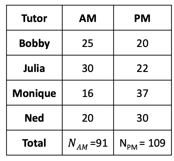
- Research question: **What is the effect of time of day (morning session vs. afternoon session) of tutoring session on midterm grades?**
- The Primary Investigator (PI) of the study wants to control for different tutor(s), believing some tutors may be better than others. Thus, they design a completely randomized block design.
- Each tutor works with students in the morning and afternoon.
- In this example, student select their favorite tutor, but are then randomly assigned to either a morning (AM) or afternoon (PM) session.
- 200 total students: 91 in the morning, 109 in the afternoon
:::
:::: {.column width="40%"}
::: callout-note
DV: Midterm Score (in cells)
:::
::::
::::::
------------------------------------------------------------------------
### Variables and Null Hypothesis
:::::: columns
::: {.column width="60%"}
- IV: Time (*a* = 2 )
- [2 levels]{style="color: orange"}: AM and PM
- Nuisance factor: Tutor (*b* = 4 )
- [4 levels]{style="color: purple"}: Booby, Julia, Monique, and Ned
- DV: Midterm Score
- Null hypothesis pertaining to the IV of interest:
- $H_0:\mu_{𝐴𝑀} = \mu_{𝑃𝑀} → a= 2$
- We will also have a null hypothesis pertaining to the blocking factor:
- $H_0:\mu_{Bobby} = \mu_{Julia} = \mu_{Monique} =\mu_{Ned} → b=4$
- Two Nulls = two values of $F_{obs}$, two values of $F_{crit}$, two decisions
:::
:::: {.column width="40%"}

::: callout-note
DV: Midterm Score (in cells)
:::
::::
::::::
------------------------------------------------------------------------
### Sum of Squares
::::: columns
::: {.column width="70%"}
- IV: Time (𝑎= 2 )
- Nuisance factor: Tutor (𝑏= 4 )
- DV: Midterm Score
- Now:
- $𝑆𝑆_{Total} =\color{red}{𝑆𝑆_{𝑀𝑜𝑑𝑒𝑙}}+\color{purple}{𝑆𝑆_{𝐵𝑙𝑜𝑐𝑘}}+\color{blue}{𝑆𝑆_{𝐸𝑟𝑟𝑜𝑟}}$
- Thus, we can partition the effects into three parts:
- Sum of squares due to [treatments (IV = Time)]{style="color: red"},
- Sum of squares due to the [blocking factor]{style="color: purple"},
- and Sum of squares due to [error]{style="color: blue"}.
- We **do not** model an **interaction** with blocked designs. (we will talk about it later.)
:::
::: {.column width="30%"}
:::
:::::
------------------------------------------------------------------------
### Mean of Squares and F-statistics
- IV: Time (𝑎= 2 )
- Nuisance factor: Tutor (𝑏= 4 )
- DV: Midterm Score
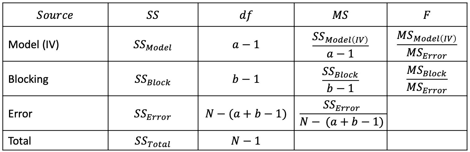
- Model: $𝑆𝑆_{Total} =\color{red}{𝑆𝑆_{𝑀𝑜𝑑𝑒𝑙}}+\color{purple}{𝑆𝑆_{𝐵𝑙𝑜𝑐𝑘}}+\color{blue}{𝑆𝑆_{𝐸𝑟𝑟𝑜𝑟}}$
- ANOVA table:
------------------------------------------------------------------------
### Sum of Square Formula
$$
SS_{\mathrm{Total}}=\sum_{i=1}^{n}(y_{ij}-\bar{y}_{..})^2
$$
- This is the same as before: take each individual score ($y_{ij}$), subtract the grand mean ($\bar{y}_{..}$), and square it $(y_{ij}-\bar{y}_{..})^2$
```{r}
scores <- c(9.1, 9.3, 9.4, 9.5) # four individuals' scores
mean(scores) # grand mean
sum((scores - mean(scores))^2) # sum of squares of total indivisuals
```
- Do this for everyone and then sum over all people $\sum_{i=1}^{n}(y_{ij}-\bar{y}_{..})^2$
- However, when calculating **S**um of **S**quares for IVs: $SS_{Model}$, $SS_{Block}$, $SS_{error}$, we need to compute "**marginal means**"
- A **marginal mean** is the mean for one level of the variable, ignoring the other variable
------------------------------------------------------------------------
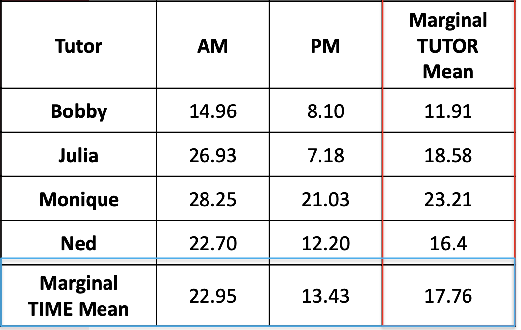
### Marginal Means
- A **marginal mean** is the mean for one level of the variable, ignoring the other variable
::::: columns
::: {.column width="50%"}
**For example**:
- The AM marginal mean is the average of all students’ midterm scores in the morning, ignoring who they have as a tutor $$
\bar{y}_{AM.} = 22.95
$$
- The Bobby marginal mean is the average of all students’ midterm scores who had Bobby as a tutor, ignoring time of day $$
\bar{y}_{.Bobby} = 11.91
$$
:::
::: {.column width="50%"}
:::
:::::
------------------------------------------------------------------------
### SS for Total and Time/Model
$$
SS_{Total} = \sum_{i=1}^{n}(y_{ij}-\bar{y}_{..})^2=15060.48
$$
$$
SS_{Model(time)} = \sum_{a=1}^{a}n_a(\bar{y}_{a.}-\bar{y}_{..})^2=4489.02
$$
- where $n_a$ is the group size for AM/PM and $\bar{y}_{a.}$ are the marginal means for AM and PM {22.95, 13.43}
- This is similar to how we computed $𝑆𝑆_{𝑀𝑜𝑑𝑒𝑙}$ before: marginal group mean subtract off the grand mean and square it. Sum over all groups.
$$
SS_{Block} = \sum_{b=1}^{b}n_{b}(\bar{y}_{.b}-\bar{y}_{..})^2=3239.43
$$
- Technically, the blocking factor is just another IV (but we are not interested in or is not within the scope of research question).
- $𝑆𝑆_{𝐸𝑟𝑟𝑜𝑟} = 𝑆𝑆_{𝑇𝑜𝑡𝑎𝑙}− 𝑆𝑆_{𝑀𝑜𝑑𝑒𝑙} +𝑆𝑆_{𝐵𝑙𝑜𝑐𝑘}$ = 7332. 03
------------------------------------------------------------------------
### Results of ANOVA Table
- Then, we can fill out the ANOVA table:
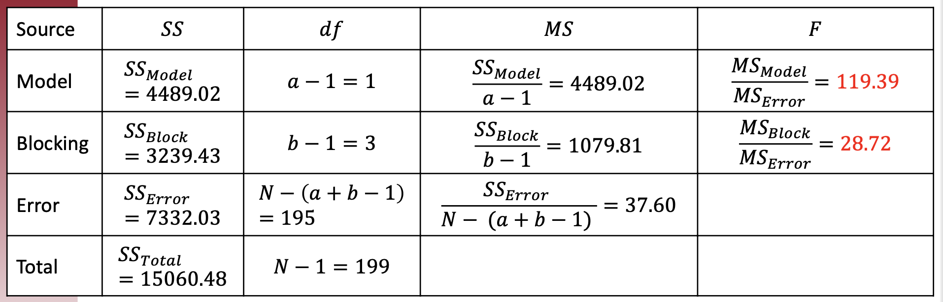
::: callout-note
Under $\alpha=.05$, for "Model" factor – Time, we have $df_{Model}$ = 1, $df_{error} = 195$: $F_{crit}=3.89$ so sig.
Similarly, for "Blocking" - Tutor, we have $df_{block}$ = 3, $df_{error} = 195$: $F_{crit}=2.65$ so sig.
:::
------------------------------------------------------------------------
### Interpretation
- A randomized block design was used to test the effect of tutoring time on midterm scores. For each tutor, participants were randomly assigned to either morning (𝑛 = 91 ) or afternoon (𝑛= 109 ) tutoring sessions.
- The effect of tutoring time was significant $(𝐹(1,195) = 119. 39, 𝑝<. 001 ,\eta^2_{𝑇𝑖𝑚𝑒} =. 298$) with a large effect. Using a Tukey’s test, morning is significantly higher than afternoon sessions (𝑝 \<. 05 ).
- The effect of the blocking factor, tutor, was significant ($𝐹(3 , 195) = 28. 72 ,𝑝< . 001 ,\eta^2_{𝑇𝑢𝑡𝑜𝑟} =. 215$) with a large effect. Using a Tukey’s test, Monique’s students were significantly higher than other students, and Bobby’s students were significantly lower than other students in the midterm scores (𝑝\<. 05 ).
## Example 3: Hardness Reading[^2]
[^2]: Please check the original post here: [STAT 503](https://online.stat.psu.edu/stat503/lesson/4/4.1)
- In this example we wish to determine whether 4 different tips (the treatment factor) produce different (mean) hardness readings on a Rockwell hardness tester.
- The **treatment factor** is the design of the tip for the machine that determines the hardness of metal. The tip is one component of the testing machine.
::: callout-note
### The Rockwell hardness test
**The Rockwell hardness test** is a hardness test based on indentation hardness of a material. The Rockwell test measures the depth of penetration of an indenter under a large load (major load) compared to the penetration made by a preload (minor load).
:::
- To conduct this experiment we assign the tips to an experimental unit; that is, to a **test specimen** (called a coupon), which is a piece of metal on which the tip is tested.
- The **blocking factor** is the block of test specimens. The test specimens are blocks of metal that are similar in hardness. The test specimens are used to block the variation in hardness of the metal from the variation in the tips.
------------------------------------------------------------------------
### Example: Block Design - CRD
- If the structure were a completely randomized experiment (CRD) that we discussed in lecture 7, we would assign the tips to a random piece of metal for each test. In this case, the test specimens would be considered a source of nuisance variability.
```{r}
#| code-fold: true
set.seed(1234)
data.frame(
  Metal = paste0("Metal", 1:8),
  Tip = rep(c("Tip1", "Tip2", "Tip3", "Tip4"), each = 2),
  Hardness = sample(seq(9, 10, by =.1), 8)
)
```
------------------------------------------------------------------------
### Example: Block Design - RCBD
- If we conduct this as a blocked experiment, we would assign all four tips to the same test specimen, randomly assigned to be tested on a different location on the specimen. Since each treatment occurs once in each block, the number of test specimens is the number of replicates.
- Back to the hardness testing example, the experimenter may very well want to *test the tips* (treatment) across *specimens* (block) of various hardness levels. This shows the importance of blocking. To conduct this experiment as a RCBD, we assign all 4 tips to each specimen.
- In this experiment, each specimen is called a “block”; thus, we have designed a more homogenous set of experimental units on which to test the tips.
------------------------------------------------------------------------
### Example: Block Design Table - RCBD
::::: columns
::: column
- Suppose that we use b = 4 blocks as shown in the table below:
- We are primarily interested in testing the equality of treatment means, but now we have the ability to remove the variability associated with the nuisance factor (the blocks) through the grouping of the experimental units prior to having assigned the treatments.
:::
::: column
```{r}
#| code-fold: true
tribble(
  ~`1`,     ~`2`,   ~`3`,   ~`4`,
  "Tip 3",  "Tip 3",    "Tip 2",    "Tip 1",
  "Tip 1",  "Tip 4",    "Tip 1",    "Tip 4",
  "Tip 4",  "Tip 2",    "Tip 3",    "Tip 3",
  "Tip 2",  "Tip 1",    "Tip 4",    "Tip 3"
) |>
  gt() |>
  tab_header(
    title = "The Hardness Testing Experiment",
    subtitle = "Randomized Complete Block Design"
  ) |>
  tab_spanner(
    label = "Test Coupon (Block)",
    columns = everything()
  ) |>
  tab_options(
    table.width = px(500),
    table.font.size = px(20)
  )
```
:::
:::::
::: callout-important
Notice the two-way structure of the experiment. Here we have four blocks and within each of these blocks is a random assignment of the tips within each block.
:::
------------------------------------------------------------------------
### Example: ANOVA Results (1)
- Remember, the hardness of specimens (coupons) is tested with 4 different tips.
```{r}
#| code-fold: true
library(here)
dat <- read.csv(here::here("teaching/2025-01-13-Experiment-Design/Lecture08", "tip_hardness.csv"))
head(dat)
```
------------------------------------------------------------------------
### Example: ANOVA Results (2)
- Here is the output from R `aov()`. We can see four levels of the Tip and four levels for Coupon:
```{r}
#| code-fold: true
dat$Tip <- factor(dat$Tip)
dat$Coupon <- factor(dat$Coupon)
fit_exp2 <- aov(Hardness ~ Tip + Coupon, data = dat)
summary(fit_exp2)
```
::: callout-note
- The Analysis of Variance table shows three degrees of freedom for Tip three for Coupon, and the residual (error) degrees of freedom is nine.
- The ratio of mean squares of treatment over error gives us an F ratio that is equal to 14.44 which is highly significant since it is greater than the .001 percentile of the F distribution with three and nine degrees of freedom.
- Our 2-way analysis also provides a test for the block factor, Coupon. The ANOVA shows that this factor is also significant with an F-test = 30.94. So, there is a large amount of variation in hardness between the pieces of metal.
- This is why we used specimen (or coupon) as our blocking factor. We expected in advance that it would account for a large amount of variation. By including block in the model and in the analysis, we removed this large portion of the variation, such that the residual error is quite small. By including a block factor in the model, the error variance is reduced, and the test on treatments is more powerful.
:::
### Example: ANOVA Results (3)
- The test on the block factor is typically not of interest except to confirm that you used a good blocking factor. The results are summarized by the table of means given below.
```{r}
#| code-fold: true
cbind(
dat |>
  group_by(Tip) |>
  summarize(
    N_Tip = n(),
    Hardness_Tip = mean(Hardness)),
dat |>
  group_by(Coupon) |>
  summarize(
    N_Coupon = n(),
    Hardness_Coupon = mean(Hardness))
)
```
## Example 4: Hours spent on the study in varied environments
- **Background:** Comparing the hours spent on the study for gender (male and female) blocks in different environments (at home and at college). To represent this experiment in the figure will be as follows:
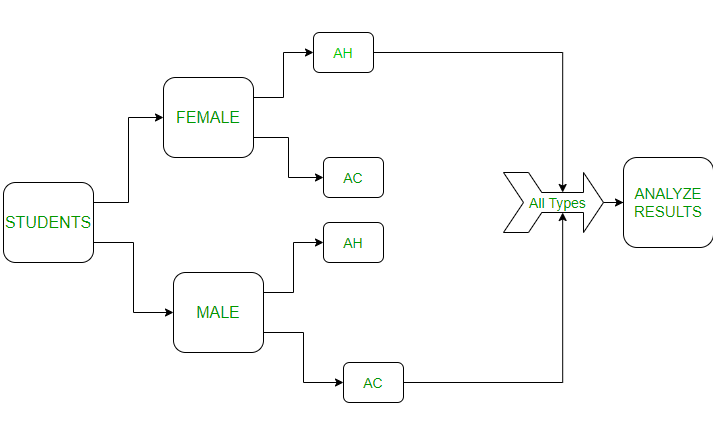
- Where *AC*: At College, *AH*: At Home
```{r}
gender <- factor(rep(c("male", "female"), each = 2))
env <- factor(rep(c("ah", "ac" ), times = 2))
y <- c(5.5, 5, 4, 6.2)
# y is the hours students
# studied in specific places
results <- data.frame(y, gender, env)
results
```
::: panel-tabset
### Exercise
Try to obtain (1) the sum of squares for treatment and block (2) F-statistics. Then, interpret the results.
```{webr-r}
gender <- factor(rep(c("male", "female"), each = 2))
env <- factor(rep(c("ah", "ac" ), times = 2))
y <- c(5.5, 5, 4, 6.2)
# y is the hours students
# studied in specific places
results <- data.frame(y, gender, env)
results
```
### Answer
```{r}
fit <- aov(y ~ gender+env, data = results)
summary(fit)
```
- **Explanation**: The value of Mean Sq is `0.7225<<1.8225`,i.e, here blocking wasn't necessary. And as Pr value is 0.642 \> 0.05 (5% significance) we fail to reject the null hypothesis - there is no sufficient evidence suggesting females and males have significant differences in performance.
:::
## Blocking factor or not?
::: discussion
### Effectiveness of Health Promotion Programs {.unnumbered}
- Researchers are interested in comparing the effectiveness of three health promotion programs with nursing students.
- The researcher has the following research question: *Which of the three health promotion programs are most effective at reducing unhealthy coping behaviors?*
1. Unhealthy coping behavior is measured as a composite score from the “Poor Coping Behavior” survey (PCB). High scores on the PCB indicate higher levels of unhealthy coping behaviors. Low scores indicate low levels of unhealthy coping behaviors. PCB scores can range from 0 (no unhealthy behaviors) to 100 (multiple unhealthy behaviors at high frequency and high intensity).
2. The researcher thinks that the health promotion programs for nursing students may have an effect on academic and well-being outcomes.
3. However, gender and status (traditional vs. non-traditional student) differences may influence the effectiveness of health promotion programs.
:::
------------------------------------------------------------------------
### Blocking Factors?
- The researcher has a sample of 200 nursing students from the state of Arkansas. 50 students are assigned to each program: Program A, Program B, and Program C. In addition, 50 students are assigned to a control group that receives the status quo educational model.
```{r}
data.frame(
  Health_Program = c("Program A", "Program B", "Program C", "Control"),
  N = c(50, 50, 50, 50)
)
```
------------------------------------------------------------------------
### Blocking Factors?
::: panel-tabset
## Visualization
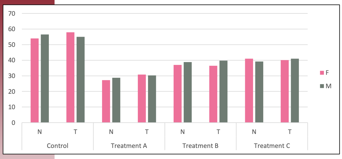
## Table
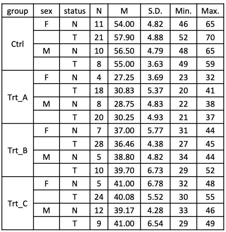
:::
------------------------------------------------------------------------
### Factors
1. What is the dependent variable? → [PCB SCORES]{.mohu}
2. What is the independent variable of interest? → [HEALTH PROGRAM (4 LEVELS)]{.mohu}
3. What is (are) the confounding variables, that the researcher might statistically control for? → [`GENDER`, `STATUS`]{.mohu}
4. What is (are) the blocking factors? → [`Schools`, `Classes`]{.mohu}
------------------------------------------------------------------------
# Wrap-up
## Summary
In this lecture, we covered:
1. **Randomized Complete Block Design (RCBD)**
- Features: Equal block sizes, random assignment within blocks, each treatment appears once per block
- Statistical model: $Y_{ij} = \mu + \tau_i + \rho_j + \epsilon_{ij}$
- Assumptions: No interaction between treatment and block factors
2. **Sum of Squares Decomposition**
- Total variation partitioned into: $SS_{Total} = SS_{Treatment} + SS_{Block} + SS_{Residual}$
- Marginal means used to calculate treatment and block effects
- F-statistics used to test treatment and block effects
3. **Benefits of Blocking**
- Reduces error variance (MSE) by removing block-to-block variation
- Increases power of F-tests for treatment effects
- More precise estimation of treatment effects
4. **Practical Examples**
- Applied RCBD to detergents, tutoring sessions, hardness testing, plant fertilizer, and study environments
- Used R's `aov()` function with formula: `Outcome ~ Treatment + Block`
- Compared RCBD results with completely randomized designs (CRD)
## Key Takeaways
::: callout-important
- **When to use RCBD**: When there are known sources of nuisance variation that can be grouped into blocks
- **Effect of blocking**: Smaller MSE leads to larger F-statistics and more powerful tests
- **Blocking effectiveness**: Check if block factor is significant to confirm it was a good blocking choice
- **Model assumptions**: No treatment-by-block interaction (additive model only)
:::
## Next Steps
- Complete [Homework 2](https://docs.google.com/forms/d/e/1FAIpQLSfXv9fBlRLaGB5eV79qfL30AVOiul7bSrMWbqns2iCz7IdgHA/viewform?usp=header)
- Practice identifying appropriate blocking factors in research scenarios
- Review sum of squares calculations and marginal means
- Prepare for more advanced blocking designs (Latin squares, factorial designs with blocks)


