---
title: "Lecture 10: Two-way ANOVA II"
subtitle: "Statistics in 2-way ANOVA"
date: "2025-03-07"
date-modified: "`{r} Sys.Date()`"
execute:
eval: true
echo: true
warning: false
message: false
webr:
editor-font-scale: 1.2
format:
html:
toc-expand: 3
code-tools: true
code-line-numbers: false
code-fold: false
code-summary: "Click to see R code"
number-offset: 1
fig.width: 10
fig-align: center
message: false
grid:
sidebar-width: 350px
uark-revealjs:
chalkboard: true
embed-resources: false
code-fold: false
number-sections: true
number-depth: 1
footer: "ESRM 64503"
slide-number: c/t
tbl-colwidths: auto
scrollable: true
output-file: slides-index.html
mermaid:
theme: forest
---
::: objectives
## Overview of Lecture 09 & Lecture 10 {.unnumbered}
1. The rest of the semester
2. Advantage of Factorial Design
3. Two-way ANOVA:
- Steps for conducting 2-way ANOVA
- Hypothesis testing
- Assumptions for 2-way ANOVA
- Visualization
- Difference between 1-way and 2-way ANOVA
**Question**: How about the research scenario when more than two independent variables?
:::
# Hypothesis testing for two-way ANOVA
## Hypothesis testing for two-way ANOVA (I)
- For two-way ANOVA, there are three distinct hypothesis tests :
- Main effect of Factor A
- Main effect of Factor B
- Interaction of A and B
::: callout-note
### Definition
F-test
: Three separate F-tests are conducted for each!
Main effect
: Occurs when there is a difference between levels for one factor
Interaction
: Occurs when the effect of one factor on the DV depends on the particular level of the other factor
: Said another way, when the difference in one factor is moderated by the other
: Said a third way, if the difference between levels of one factor is different, depending on the other factor
:::
## Hypothesis testing for two-way ANOVA (II)
1. Hypothesis test for the main effect with more than 2 levels
- Mean differences among levels of one factor:
i) Differences are tested for statistical significance
ii) Each factor is evaluated independently of the other factor(s) in the study
- Factor A’s Main effect: “Controlling Factor B, are there differences in the DV across Factor A?”
$H_0$: $\mu_{A_1}=\mu_{A_2}=\cdots=\mu_{A_k}$
$H_1$: At least one $\mu_{A_i}$ is different from the control group in Factor A
- Factor B’s Main effect : “Controlling Factor A, are there differences in the DV across Factor B?”
$H_0$: $\mu_{B_1}=\mu_{B_2}=\cdots=\mu_{B_k}$
$H_1$: At least one $\mu_{B_i}$ is different from the control group in Factor A
- Interaction effect between A and B:
$H_0:\mu_{A_1B_2}-\mu_{A_1B_1}=\mu_{A_2B_2}-\mu_{A_2B_1}$
or $H_0: \mu_{A_1B_1}-\mu_{A_2B_1}=\mu_{A_1B_2}-\mu_{A_2B_2}$
::: rmdnote
**The null hypothesis of interaction**: B's group differences do not change across different levels of A. OR A's group differences do not change at different levels of B.
:::
## Hypothesis testing for two-way ANOVA (III)
::: callout-important
## Example
**Background**: A researcher is investigating how study method (Factor A: Lecture vs. Interactive) and test format (Factor B: Multiple-Choice vs. Open-Ended) affect student performance (dependent variable: test scores). The study involves randomly assigning students to one of the two study methods and then assessing their performance on one of the two test formats.
- **Main Effect of Study Method (Factor A):**
- [H0:]{style="color:royalblue; font-weight:bold"} There is no difference in test scores between students who used the Lecture method and those who used the Interactive method.
- [H1:]{style="color:tomato; font-weight:bold"} There is a significant difference in test scores between the two study methods.
- **Main Effect of Test Format (Factor B):**
- [H0:]{style="color:royalblue; font-weight:bold"} There is no difference in test scores between students taking a Multiple-Choice test and those taking an Open-Ended test.
- [H1:]{style="color:tomato; font-weight:bold"} There is a significant difference in test scores between the two test formats.
- **Interaction Effect (Study Method × Test Format):**
- [H0:]{style="color:royalblue; font-weight:bold"} The effect of study method on test scores is the same regardless of test format.
- [H1:]{style="color:tomato; font-weight:bold"} The effect of study method on test scores depends on the test format (i.e., there is an interaction).
:::
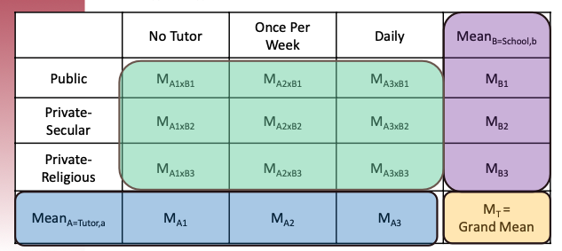
## Hypothesis testing for two-way ANOVA (IV)
::: callout-note
### Example: Tutoring Program and Types of Schools on Grades
- **IVs**:
1. Tutoring Programs: (1) No tutor; (2) Once a week; (3) Daily
2. Types of schools: (1) Public (2) Private-secular (3) Private-religious
- **Research purpose**: to examine the effect of tutoring program (no tutor, once a week, and daily) AND types of school (e.g., public, private-secular, and private-religious) on the students’ grades
- **Question**: What are the null and alternative hypotheses for the main effects in the example?:
- Factor A’s Main effect: “[Controlling school types, are there differences in the students’ grade across three tutoring programs?]{.mohu}”
$H_0$: $\mu_{\mathrm{no\ tutor}}=\mu_{\mathrm{once\ a\ week}}=\mu_{\mathrm{daily}}$
- Factor B’s Main effect : “[Controlling tutoring programs, are there differences in the students’ grades across three school types?]{.mohu}”
$H_0$: $\mu_{\mathrm{public}}=\mu_{\mathrm{private-religious}}=\mu_{\mathrm{private-secular}}$
:::
## Model 1: Two-Way ANOVA without interaction
- The main-effect only ANOVA with no interaction has a following statistical form:
$$
\mathrm{Grade} = \beta_0 + \beta_1 \mathrm{Toturing_{Once}} + \beta_2 \mathrm{Toturing_{Daily}} \\ + \beta_3 \mathrm{SchoolType_{PvtS}} + \beta_4 \mathrm{SchoolType_{PvtR}}
$$
```{webr-r}
#| context: setup
library(tidyverse)
# Set seed for reproducibility
set.seed(123)
# Define sample size per group
n <- 30
# Define factor levels
tutoring <- rep(c("No Tutor", "Once a Week", "Daily"), each = 3 * n)
school <- rep(c("Public", "Private-Secular", "Private-Religious"), times = n * 3)
# Simulate student grades with assumed effects
grades <- c(
rnorm(n, mean = 75, sd = 5), # No tutor, Public
rnorm(n, mean = 78, sd = 5), # No tutor, Private-Secular
rnorm(n, mean = 76, sd = 5), # No tutor, Private-Religious
rnorm(n, mean = 80, sd = 5), # Once a week, Public
rnorm(n, mean = 83, sd = 5), # Once a week, Private-Secular
rnorm(n, mean = 81, sd = 5), # Once a week, Private-Religious
rnorm(n, mean = 85, sd = 5), # Daily, Public
rnorm(n, mean = 88, sd = 5), # Daily, Private-Secular
rnorm(n, mean = 86, sd = 5) # Daily, Private-Religious
)
# Create a data_frame
data <- data.frame(
Tutoring = factor(tutoring, levels = c("No Tutor", "Once a Week", "Daily")),
School = factor(school, levels = c("Public", "Private-Secular", "Private-Religious")),
Grades = grades
)
```
```{r}
#| eval: true
#| code-fold: true
#| code-summary: "Data Generation"
library(tidyverse)
# Set seed for reproducibility
set.seed(123)

# Define sample size per group
n <- 30

# Define factor levels
tutoring <- rep(c("No Tutor", "Once a Week", "Daily"), each = 3 * n)
school <- rep(c("Public", "Private-Secular", "Private-Religious"), times = n * 3)

# Simulate student grades with assumed effects
grades <- c(
  rnorm(n, mean = 75, sd = 5),  # No tutor, Public
  rnorm(n, mean = 78, sd = 5),  # No tutor, Private-Secular
  rnorm(n, mean = 76, sd = 5),  # No tutor, Private-Religious
  rnorm(n, mean = 80, sd = 5),  # Once a week, Public
  rnorm(n, mean = 83, sd = 5),  # Once a week, Private-Secular
  rnorm(n, mean = 81, sd = 5),  # Once a week, Private-Religious
  rnorm(n, mean = 85, sd = 5),  # Daily, Public
  rnorm(n, mean = 88, sd = 5),  # Daily, Private-Secular
  rnorm(n, mean = 86, sd = 5)   # Daily, Private-Religious
)
# Create a dataframe
data <- data.frame(
  Tutoring = factor(tutoring, levels = c("No Tutor", "Once a Week", "Daily")),
  School = factor(school, levels = c("Public", "Private-Secular", "Private-Religious")),
  Grades = grades
)
```
- Main effect of Tutoring Programs
- Collapsing across School Type
- Ignoring the difference levels of School Type
- Averaging DV regarding Tutoring Programs across the levels of School Type
- Main effect of School Type
- Collapsing across Tutoring Program
- Ignoring the difference levels of Tutoring Program
- Averaging DV regarding School Type across the levels of Tutoring Programs
------------------------------------------------------------------------
::: panel-tabset
### R Plot
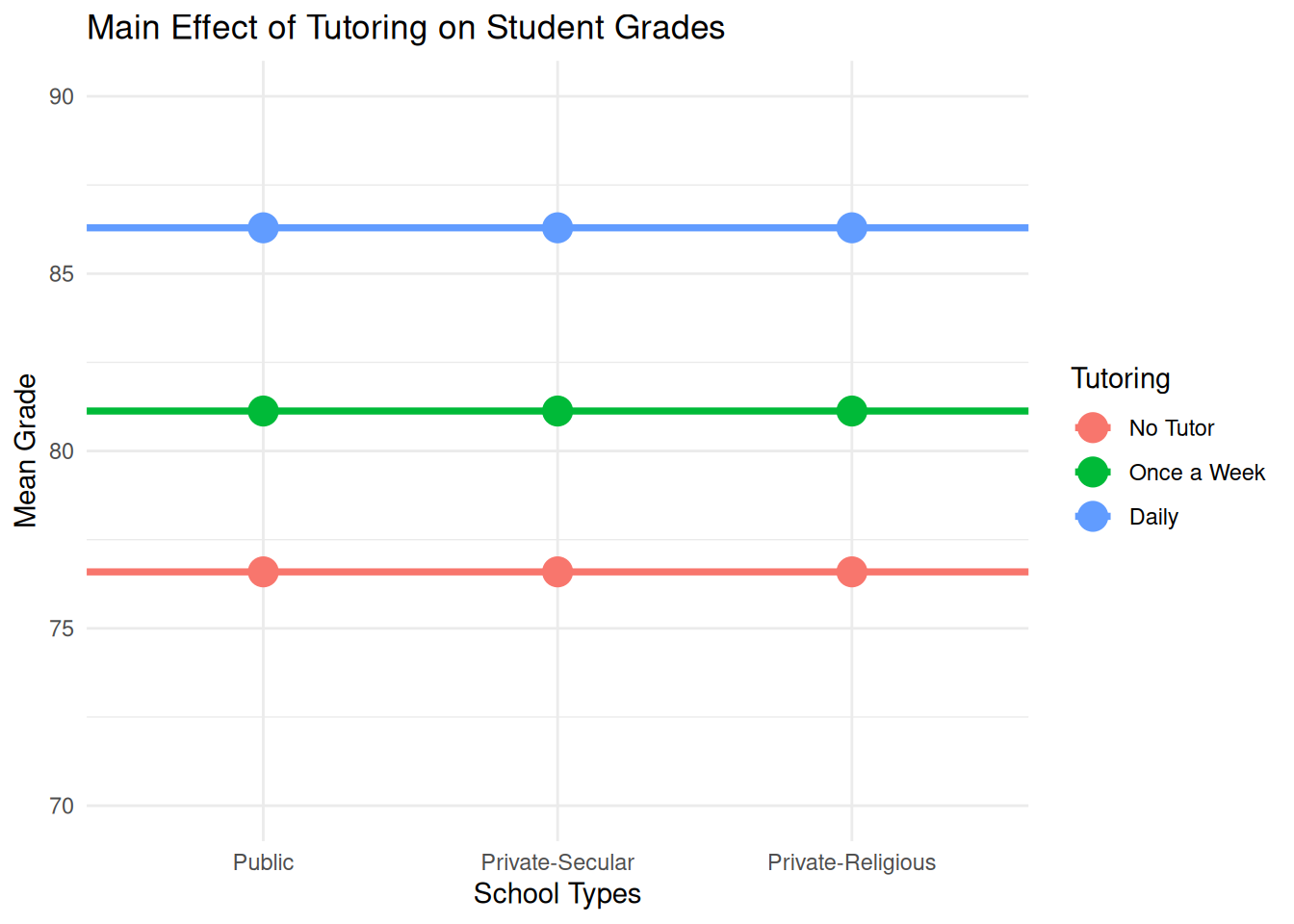
Ignoring the effect of school types, we can tell the main effect of tutor programs on students' grades (Daily tutoring has the highest grade, followed by *once a week*).
```{r}
#| code-fold: true
# Compute mean and standard error for each tutoring group
tutoring_summary <- data |>
  group_by(Tutoring) |>
  summarise(
    Mean_Grade_byTutor = mean(Grades)
  )

school_summary <- data |>
  group_by(School) |>
  summarise(
    Mean_Grade_bySchool = mean(Grades)
  )

total_summary <- tutoring_summary |>
  cbind(school_summary)

# Plot main effect of tutoring
ggplot(total_summary, aes(x = School)) +
  geom_point(aes(y = Mean_Grade_byTutor, color = Tutoring), size = 5) +
  geom_hline(aes(yintercept = Mean_Grade_byTutor, color = Tutoring), linewidth = 1.3) +
  scale_y_continuous(limits = c(70, 90), breaks = seq(70, 90, 5)) +
  labs(title = "Main Effect of Tutoring on Student Grades",
       x = "School Types",
       y = "Mean Grade") +
  theme_minimal()
```
### Summary Statistics
```{r}
distinct(tutoring_summary[, c("Tutoring", "Mean_Grade_byTutor")])
```
### Interpretation of the Plot
- The x-axis represents three school types.
- The y-axis represents the mean student grades for the different tutoring programs: No Tutor, Once a Week, and Daily.
- If the main effect of tutoring is significant, we expect to see noticeable differences in mean grades across tutoring conditions.
:::
## You turn: Visualize Main Effect of School Type
::: panel-tabset
### Marginal Means for each tutoring / school type group
```{webr-r}
School_Levels <- c("Public",
"Private-Secular",
"Private-Religious")
## Calculate marginal means for tutoring
tutoring_summary <- data |>
group_by(Tutoring) |>
summarise(
Mean_Grade_byTutor = mean(Grades)
) |>
mutate(School = factor(School_Levels,
levels = School_Levels))
## Calculate marginal means for school types
school_summary <- data |>
group_by(School) |>
summarise(
Mean_Grade_bySchool = mean(Grades)
)
## Combine them into one table
total_summary <- tutoring_summary |>
left_join(school_summary, by = "School")
```
### Plot main effect of School Type
```{webr-r}
ggplot(total_summary, aes(x = Tutoring)) +
geom_point(aes(y = Mean_Grade_bySchool, color = School)) +
geom_hline(aes(yintercept = Mean_Grade_bySchool, color = School), linewidth = 1.3) +
scale_y_continuous(limits = c(70, 90), breaks = seq(70, 90, 5)) +
labs(title = "Main Effect of School Type on Student Grades",
x = "Tutoring Type",
y = "Mean Grade") +
theme_minimal() +
theme(legend.position = "none") # Remove legend for cleaner visualization
```
:::
## Combined Visualization for no-interaction model
::: panel-tabset
### R Plot
```{webr-r}
fit <- lm(Grades ~ Tutoring + School, data = data)
Line_No_Tutor <- c(fit$coefficients[1], fit$coefficients[1] + c(fit$coefficients[4], fit$coefficients[5]))
Line_Once_A_Week <- Line_No_Tutor + fit$coefficients[2]
Line_Daily <- Line_No_Tutor + fit$coefficients[3]
School_Levels <- c("Public","Private-Secular", "Private-Religious")
combined_vis_data <- data.frame(
School_Levels,
Line_No_Tutor,
Line_Once_A_Week,
Line_Daily
)
ggplot(data = combined_vis_data, aes(x = School_Levels)) +
geom_path(aes(y = as.numeric(Line_No_Tutor)), group = 1, color = "red", linewidth = 1.4) +
geom_path(aes(y = as.numeric(Line_Once_A_Week)), group = 1, color = "green", linewidth = 1.4) +
geom_path(aes(y = as.numeric(Line_Daily)), group = 1, color = "blue", linewidth = 1.4) +
geom_point(aes(y = as.numeric(Line_No_Tutor))) +
geom_point(aes(y = as.numeric(Line_Once_A_Week))) +
geom_point(aes(y = as.numeric(Line_Daily))) +
labs(title = "Main Effect of Tutoring and School Type on Student Grades",
x = "Tutoring Type",
y = "Mean Grade") +
theme_minimal() +
theme(legend.position = "none")
```
### In the graph
- There is the LARGE effect of Factor [Tutoring]{.mohu} and very small effect of [School Type]{.mohu}:
- Effect of Factor [Tutoring]{.mohu}: the LARGE vertical distance
- Effect of Factor [School Type]{.mohu}: the very small horizontal distance
:::
## Real-World Examples of Interaction Effects
::: panel-tabset
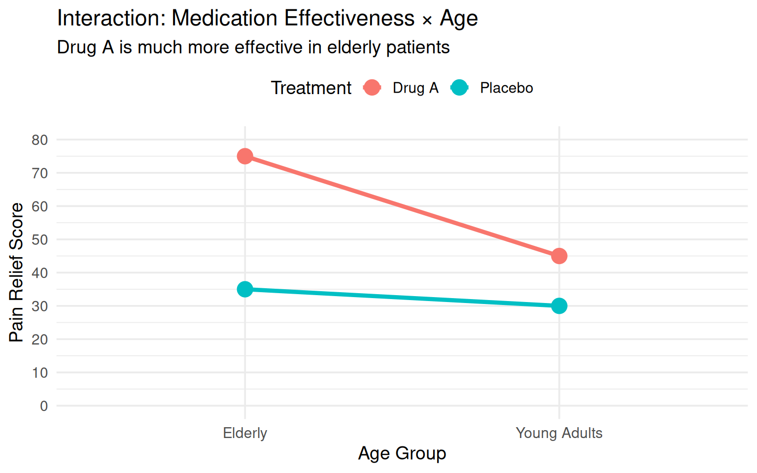
#### Example 1: Medication & Age
**Research Question**: Does the effectiveness of a new pain medication depend on patient age?
**Factors:**
- Factor A: Medication Type (Drug A vs. Placebo)
- Factor B: Age Group (Young Adults vs. Elderly)
**Observed Pattern (Interaction Present):**
- **Young Adults**: Drug A shows moderate improvement over placebo (Δ = 15 points)
- **Elderly**: Drug A shows LARGE improvement over placebo (Δ = 40 points)
**Why the interaction?**
- Elderly patients may have different metabolism rates
- Age-related changes in pain receptors may make them more responsive to the drug
- Elderly may have more severe baseline pain, allowing more room for improvement
**Implication**: You cannot simply say "Drug A works" - you must specify "Drug A works **especially well** for elderly patients"
**Visualization:**
```{r}
#| echo: false
#| fig-width: 8
#| fig-height: 5
library(ggplot2)
medication_data <- data.frame(
Age = rep(c("Young Adults", "Elderly"), each = 2),
Treatment = rep(c("Placebo", "Drug A"), 2),
Pain_Relief = c(30, 45, 35, 75)
)
ggplot(medication_data, aes(x = Age, y = Pain_Relief, color = Treatment, group = Treatment)) +
geom_point(size = 5) +
geom_line(linewidth = 1.5) +
labs(title = "Interaction: Medication Effectiveness × Age",
subtitle = "Drug A is much more effective in elderly patients",
x = "Age Group",
y = "Pain Relief Score",
color = "Treatment") +
theme_minimal(base_size = 14) +
scale_y_continuous(limits = c(0, 80), breaks = seq(0, 80, 10)) +
theme(legend.position = "top")
```
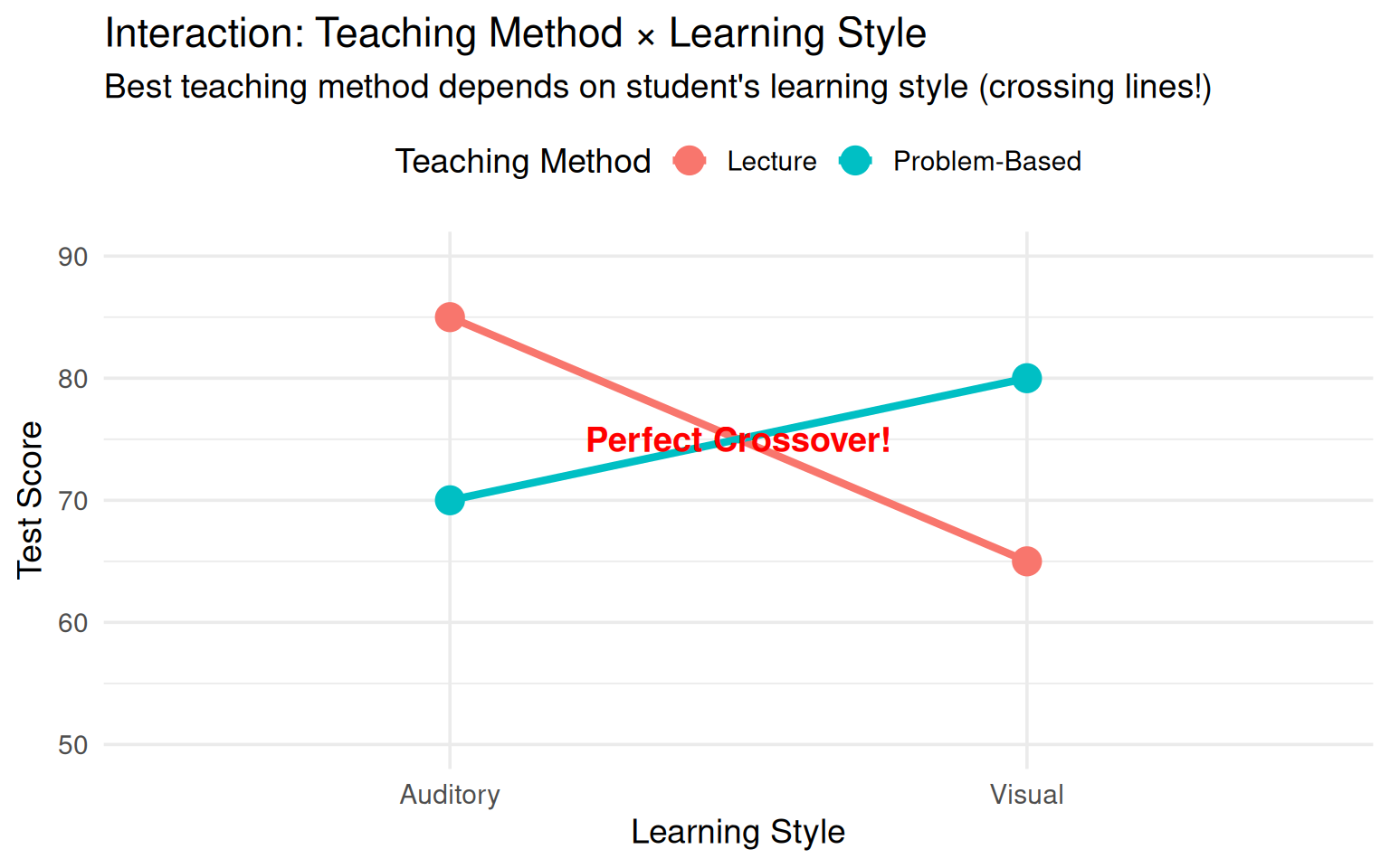
#### Example 2: Teaching Method & Learning Style
**Research Question**: Does the best teaching method depend on students' learning style?
**Factors:**
- Factor A: Teaching Method (Lecture-Based vs. Problem-Based Learning)
- Factor B: Learning Style (Visual vs. Auditory Learners)
**Observed Pattern (Interaction Present):**
- **Visual Learners**: Problem-Based Learning \>\> Lecture-Based (80 vs. 65)
- **Auditory Learners**: Lecture-Based \>\> Problem-Based Learning (85 vs. 70)
**Why the interaction?**
- Visual learners benefit from hands-on activities with diagrams and visual aids in PBL
- Auditory learners benefit from verbal explanations and discussions in lectures
- One-size-fits-all teaching ignores individual differences in cognitive processing
**Implication**: Educational policy should consider **matching** teaching methods to learning styles, not universally adopting one method.
**Visualization:**
```{r}
#| echo: false
#| fig-width: 8
#| fig-height: 5
teaching_data <- data.frame(
Learning_Style = rep(c("Visual", "Auditory"), each = 2),
Method = rep(c("Lecture", "Problem-Based"), 2),
Test_Score = c(65, 80, 85, 70)
)
ggplot(teaching_data, aes(x = Learning_Style, y = Test_Score, color = Method, group = Method)) +
geom_point(size = 5) +
geom_line(linewidth = 1.5) +
labs(title = "Interaction: Teaching Method × Learning Style",
subtitle = "Best teaching method depends on student's learning style (crossing lines!)",
x = "Learning Style",
y = "Test Score",
color = "Teaching Method") +
theme_minimal(base_size = 14) +
scale_y_continuous(limits = c(50, 90), breaks = seq(50, 90, 10)) +
theme(legend.position = "top") +
annotate("text", x = 1.5, y = 75, label = "Perfect Crossover!",
size = 5, color = "red", fontface = "bold")
```
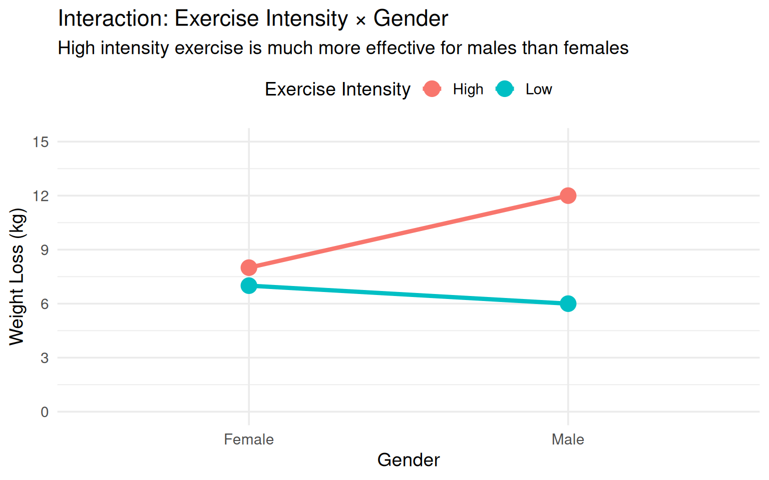
#### Example 3: Exercise & Gender
**Research Question**: Does the effect of exercise intensity on weight loss depend on biological sex?
**Factors:**
- Factor A: Exercise Intensity (Low vs. High Intensity)
- Factor B: Gender (Male vs. Female)
**Observed Pattern (Interaction Present):**
- **Males**: High intensity \>\> Low intensity (12 kg vs. 6 kg lost)
- **Females**: High intensity ≈ Low intensity (8 kg vs. 7 kg lost)
**Why the interaction?**
- Males typically have higher muscle mass and testosterone, enabling better response to high-intensity training
- Females may have hormonal differences affecting metabolism response to exercise intensity
- High-intensity exercise may increase cortisol more in females, potentially interfering with weight loss
- Different fat distribution patterns between sexes respond differently to exercise intensity
**Implication**: Exercise prescriptions should be **sex-specific**, not generic.
**Visualization:**
```{r}
#| echo: false
#| fig-width: 8
#| fig-height: 5
exercise_data <- data.frame(
Gender = rep(c("Male", "Female"), each = 2),
Intensity = rep(c("Low", "High"), 2),
Weight_Loss = c(6, 12, 7, 8)
)
ggplot(exercise_data, aes(x = Gender, y = Weight_Loss, color = Intensity, group = Intensity)) +
geom_point(size = 5) +
geom_line(linewidth = 1.5) +
labs(title = "Interaction: Exercise Intensity × Gender",
subtitle = "High intensity exercise is much more effective for males than females",
x = "Gender",
y = "Weight Loss (kg)",
color = "Exercise Intensity") +
theme_minimal(base_size = 14) +
scale_y_continuous(limits = c(0, 15), breaks = seq(0, 15, 3)) +
theme(legend.position = "top")
```
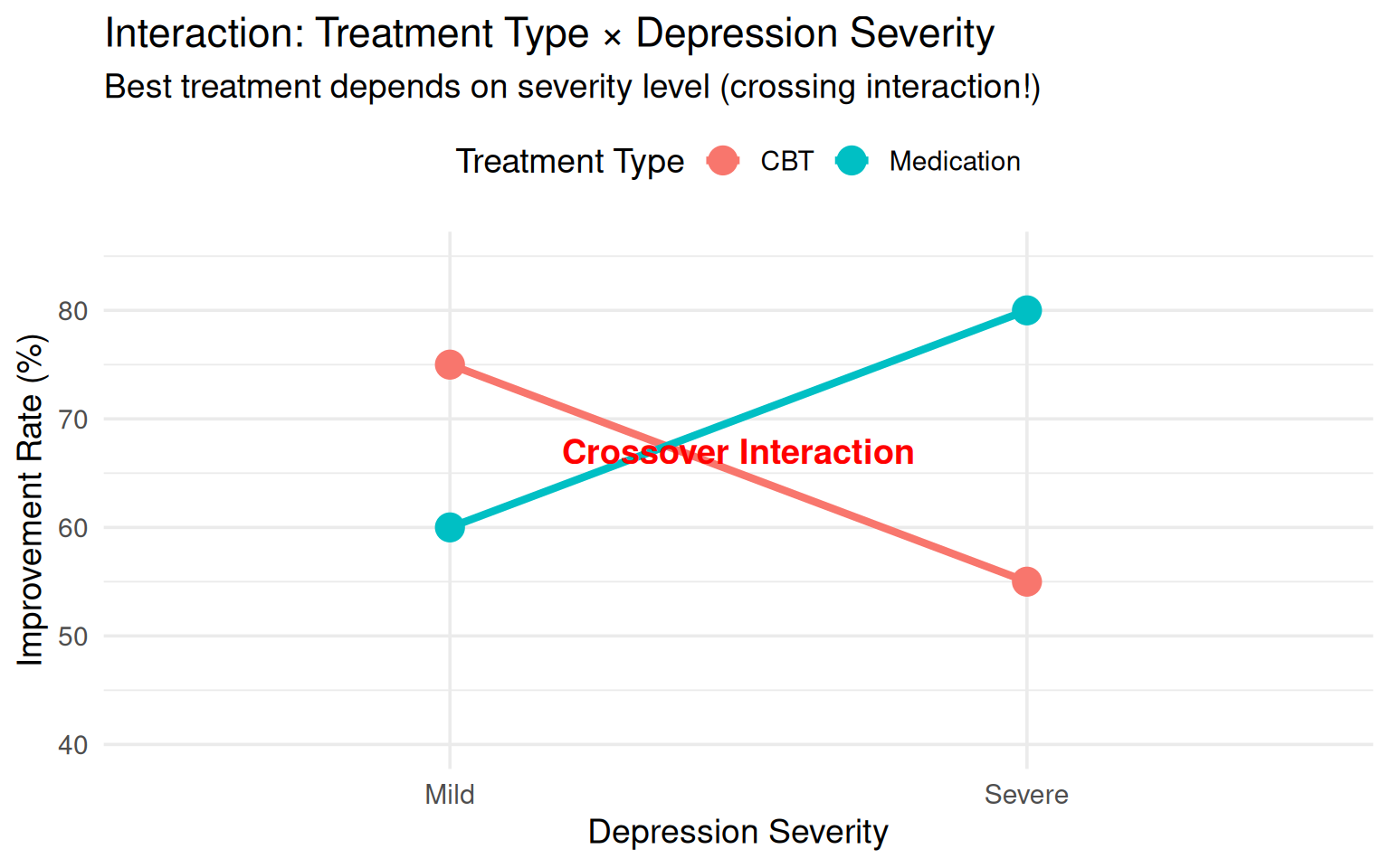
#### Example 4: Therapy & Severity
**Research Question**: Does the effectiveness of therapy type depend on depression severity?
**Factors:**
- Factor A: Therapy Type (CBT vs. Medication)
- Factor B: Depression Severity (Mild vs. Severe)
**Observed Pattern (Interaction Present):**
- **Mild Depression**: CBT \>\> Medication (75% vs. 60% improvement)
- **Severe Depression**: Medication \>\> CBT (80% vs. 55% improvement)
**Why the interaction?**
- Mild depression patients can engage effectively with cognitive strategies in CBT
- Severe depression patients may lack energy/motivation for CBT homework
- Severe cases need biological intervention (medication) to restore neurochemical balance
- CBT requires cognitive capacity that may be impaired in severe depression
**Implication**: Treatment selection should be **severity-matched**, not preference-based alone.
**Visualization:**
```{r}
#| echo: false
#| fig-width: 8
#| fig-height: 5
therapy_data <- data.frame(
Severity = rep(c("Mild", "Severe"), each = 2),
Treatment = rep(c("CBT", "Medication"), 2),
Improvement = c(75, 60, 55, 80)
)
ggplot(therapy_data, aes(x = Severity, y = Improvement, color = Treatment, group = Treatment)) +
geom_point(size = 5) +
geom_line(linewidth = 1.5) +
labs(title = "Interaction: Treatment Type × Depression Severity",
subtitle = "Best treatment depends on severity level (crossing interaction!)",
x = "Depression Severity",
y = "Improvement Rate (%)",
color = "Treatment Type") +
theme_minimal(base_size = 14) +
scale_y_continuous(limits = c(40, 85), breaks = seq(40, 85, 10)) +
theme(legend.position = "top") +
annotate("text", x = 1.5, y = 67, label = "Crossover Interaction",
size = 5, color = "red", fontface = "bold")
```
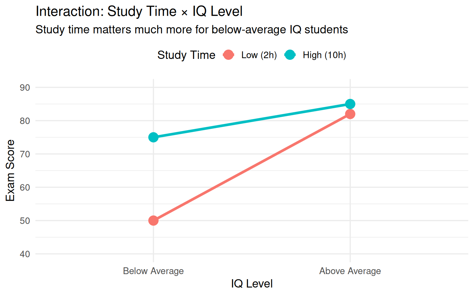
#### Example 5: Study Time & IQ
**Research Question**: Does the effect of study time on exam performance depend on intelligence level?
**Factors:**
- Factor A: Study Time (Low: 2 hrs vs. High: 10 hrs)
- Factor B: IQ Level (Below Average vs. Above Average)
**Observed Pattern (Interaction Present):**
- **Below Average IQ**: High study time \>\> Low study time (75 vs. 50 points)
- **Above Average IQ**: High study time ≈ Low study time (85 vs. 82 points)
**Why the interaction?**
- High IQ students can learn material efficiently with less study time
- Below average IQ students need more repetition and practice (more study time helps significantly)
- High IQ students may reach a "ceiling effect" - already performing well with minimal study
- Different cognitive abilities create different learning curves
**Implication**: Educational interventions (increasing study time) may be most beneficial for students who struggle, not top performers.
**Visualization:**
```{r}
#| echo: false
#| fig-width: 8
#| fig-height: 5
study_data <- data.frame(
IQ_Level = rep(c("Below Average", "Above Average"), each = 2),
Study_Time = rep(c("Low (2h)", "High (10h)"), 2),
Exam_Score = c(50, 75, 82, 85)
)
study_data$IQ_Level <- factor(study_data$IQ_Level, levels = c("Below Average", "Above Average"))
study_data$Study_Time <- factor(study_data$Study_Time, levels = c("Low (2h)", "High (10h)"))
ggplot(study_data, aes(x = IQ_Level, y = Exam_Score, color = Study_Time, group = Study_Time)) +
geom_point(size = 5) +
geom_line(linewidth = 1.5) +
labs(title = "Interaction: Study Time × IQ Level",
subtitle = "Study time matters much more for below-average IQ students",
x = "IQ Level",
y = "Exam Score",
color = "Study Time") +
theme_minimal(base_size = 14) +
scale_y_continuous(limits = c(40, 90), breaks = seq(40, 90, 10)) +
theme(legend.position = "top")
```
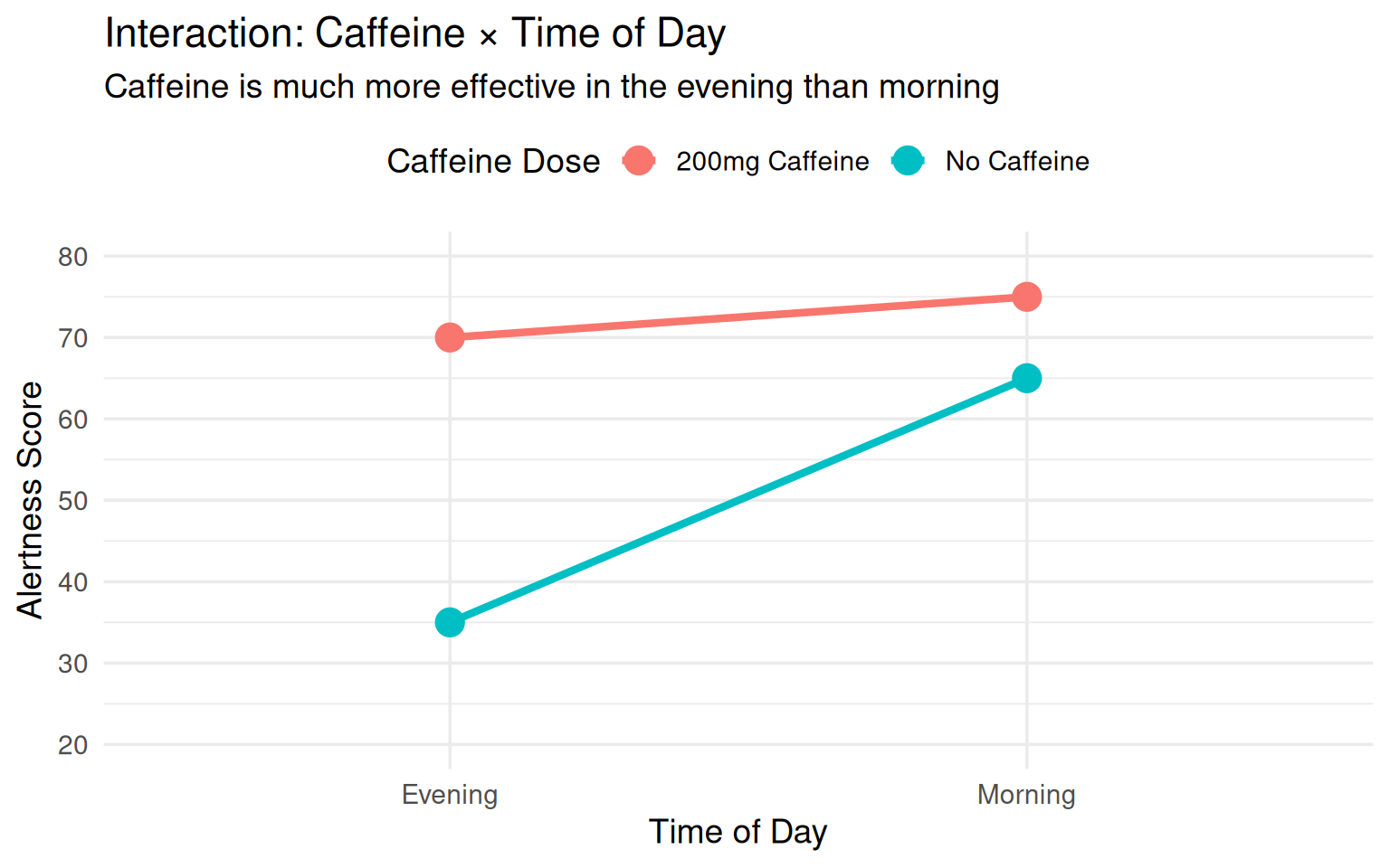
#### Example 6: Caffeine & Time of Day
**Research Question**: Does caffeine's effect on alertness depend on time of day?
**Factors:**
- Factor A: Caffeine Dose (0 mg vs. 200 mg)
- Factor B: Time of Day (Morning vs. Evening)
**Observed Pattern (Interaction Present):**
- **Morning**: Small caffeine effect (alertness: 65 vs. 75)
- **Evening**: Large caffeine effect (alertness: 35 vs. 70)
**Why the interaction?**
- Morning: Natural cortisol levels are already high (circadian rhythm), so caffeine adds less
- Evening: Cortisol levels drop naturally, so caffeine has a larger stimulating effect
- Adenosine (sleepiness molecule) accumulates throughout the day - caffeine blocks adenosine receptors
- Baseline alertness differs dramatically by time of day
**Implication**: Timing caffeine intake strategically (avoiding morning when cortisol is high) may be more effective.
**Visualization:**
```{r}
#| echo: false
#| fig-width: 8
#| fig-height: 5
caffeine_data <- data.frame(
Time = rep(c("Morning", "Evening"), each = 2),
Caffeine = rep(c("No Caffeine", "200mg Caffeine"), 2),
Alertness = c(65, 75, 35, 70)
)
ggplot(caffeine_data, aes(x = Time, y = Alertness, color = Caffeine, group = Caffeine)) +
geom_point(size = 5) +
geom_line(linewidth = 1.5) +
labs(title = "Interaction: Caffeine × Time of Day",
subtitle = "Caffeine is much more effective in the evening than morning",
x = "Time of Day",
y = "Alertness Score",
color = "Caffeine Dose") +
theme_minimal(base_size = 14) +
scale_y_continuous(limits = c(20, 80), breaks = seq(20, 80, 10)) +
theme(legend.position = "top")
```
:::
## Common Themes: Why Interactions Occur
::: callout-note
### Underlying Mechanisms for Interactions
1. **Biological Differences**: Age, sex, genetics create different physiological responses
2. **Baseline/Ceiling Effects**: Different starting points or maximum capacities across groups
3. **Mechanism Differences**: Treatments work through different pathways in different populations
4. **Resource Allocation**: Limited cognitive/physical resources are used differently across contexts
5. **Moderating Variables**: Third variables (not measured) that correlate with factors
6. **Compensatory Strategies**: Different groups adapt differently to interventions
7. **Dose-Response Variation**: Sensitivity to "dosage" varies across groups
:::
------------------------------------------------------------------------
::: callout-warning
### Critical Insight
**Ignoring interactions leads to incorrect conclusions!**
If you only report main effects in these examples, you would conclude:
- "Drug A works" (missing that it works mainly for elderly)
- "Problem-based learning is better" (missing that it depends on learning style)
- "High intensity exercise is better" (missing that it mainly benefits males)
**Always test and visualize interactions before interpreting main effects!**
:::
## Model 2: Two-Way ANOVA with Interaction
$$
\mathrm{Grade} = U_1(\mathrm{Tutoring}) + U_2(\mathrm{School}) + U_3(\mathrm{TutoringxSchool})
$$
There variance components (random effects) included in a full two-way ANOVA with two Factors.
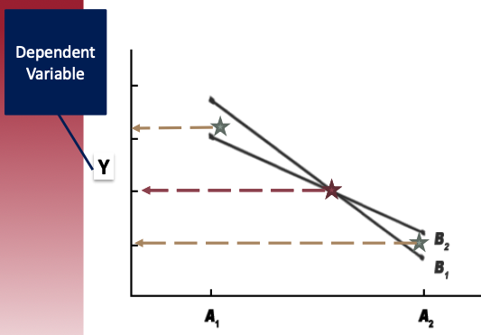
## Model 2: Visualization of Two-Way ANOVA with Interaction
::::: columns
::: column
:::
::: column
In the graph:
- There is the **LARGE** effect of Factor A and very small effect of Factor B:
- Effect of Factor A: the LARGE distance between two green stars
- Effect of Factor B: the very small distance between two red stars
In the graph, there is an intersection between two lines → This is an interaction effect between two factors!
- The level of Factor B depends upon the level of Factor A – B1 is higher than B2 for A1, but lower for A2 – B2 is lower than B1 for A1, but higher for A2
:::
:::::
# Statistical foundations of 2-way ANOVA
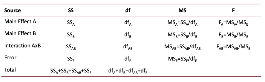
## F-statistics for Two-Way ANOVA
## F-statistics for Two-Way ANOVA: R code
::: panel-tabset
### R Code
```{webr-r}
summary(aov(Grades ~ Tutoring + School + Tutoring:School, data = data))
# or summary(aov(Grades ~ Tutoring*School, data = data))
```
### Interpretation
| Source | df | MS | F |
|------------------|------------------|------------------|------------------|
| Main Effect of Tutoring | 2 | $2120.1 = 4240 / 2$ | 89.065\*\*\* |
| Main Effect of School | 2 | $10.8 = 22 / 2$ | 0.636 |
| Interaction Effect of School x Tutoring | 4 | $46.5 = 186 / 4$ | 0.102 |
| Residual | 261 | $23.8 = 6213 / 261$ | --- |
:::
## F-statistics for Two-Way ANOVA: Degree of Freedom
- IVs:
1. Tutoring Programs: (1) No tutor; (2) Once a week; (3) Daily
2. Types of schools: (1) Public (2) Private-secular (3) Private-religious
- Degree of freedom (DF):
- $df_{tutoring}$ = (Number of levels of Tutoring) - 1 = 3 - 1 = 2
- $df_{school}$ = (Number of levels of School) - 1 = 3 - 1 = 2
- $df_{interaction}$ = $df_{tutoring} \times df_{school}$ = $2 \times 2$ = 4
- $df_{total}$ = 270 - 1 = 269
- $df_{residual}$ = $df_{total}-df_{tutoring}-df_{school} - df_{interaction}$ = 269 - 2 - 2 - 4= 261
::: callout-note
### Calculation of p-values
Based on DF and observed F statistics, we can locate observed F-statistic onto the F-distribution can calculate the p-values.
:::
## F-statistics for Two-Way ANOVA: SS and DF
Why residual DF is calculated by subtracting the total DFs with effects' DFs?
Because DF is linked to SS.
| Source | SS | df |
|----|----|----|
| Main Effect of Tutoring | 4240 | 2 |
| Main Effect of School | 22 | 2 |
| Interaction Effect of School x Tutoring | 186 | 4 |
| Residual | 6213 | 261 |
| Total | 4240 + 22 + 186 + 6213 | 2 + 2 + 4 + 261 |
```{r}
#| results: hold
sum((data$Grades - mean(data$Grades))^2) # manually calculate total Sum of squares
nrow(data) - 1 # nrow() calculate the number of rows / observations
```
```{r}
#| results: hold
4240 + 22 + 186 + 6213
2 + 2 + 4 + 261
```
## Difference between one-way and two-way ANOVA
::::: columns
::: column
### One-way ANOVA {.unnumbered}
Total = Between + Within
:::
::: column
### Two-way ANOVA {.unnumbered}
Total = FactorA + FactorB + A\*B + Residual
:::
:::::
::: rmdnote
*Within*-factor effects (one-way ANOVA) and *Residuals* (two-way ANOVA) have same meaning, both of which are unexplained part of DV by the model.
:::
- In Factor ANOVA Design, the overall between-group variability is divided up into variance terms for each unique source of the factors.
| Source | 2 IVs | 3 IVs | 4 IVs |
|------------------|------------------|------------------|------------------|
| Main effect | A, B | A, B, C | A, B, C, D |
| Interaction effect | AB | AB, BC, AC, ABC | AB, AC, AD, BC, BD, CD, ABC, ABD, BCD, ACD, ABCD |
::: macwindow
**Calculate the number of interaction effects** $$
\mathrm{N_{interaction}} = \sum_{j=2}^J C_J^j
$$
```{r}
##Number of interaction for 4 IVs
choose(4, 2) + choose(4, 3) + choose(4, 4)
```
:::
## F-statistics for Two-way ANOVA: F values
- F-observed values:
- Main effect of factor A: $F_A = \frac{SS_A/df_A}{SS_E/df_E} = \frac{MS_A}{MS_E}$
- $F_{tutoring} = \frac{MS_{tutoring}}{MS_{residual}} = \frac{2120.1}{23.8} = 89.065$
- Main effect of factor B: $F_B = \frac{MS_B}{MS_E}$
- $F_{School} = \frac{MS_{School}}{MS_{residual}} = \frac{10.8}{23.8} = 0.453$
- Interaction effect of AxB: $F_{AB} = \frac{MS_{AB}}{MS_E}$
- $F_{SxT} = \frac{MS_{SxT}}{MS_{residual}} = \frac{46.5}{23.8} = 1.953$
- Degree of freedom:
- $df_{tutoring}$ = (Number of levels of Tutoring) - 1
- $df_{school}$ = (Number of levels of School) - 1
- $df_{interaction}$ = $df_{tutoring} \times df_{school}$
- $df_{total}$ = N - 1
- $df_{residual}$ = $df_{total}-df_{tutoring}-df_{school} - df_{interaction}$
------------------------------------------------------------------------
## Exercise
- A new samples with N = 300
- Tutoring still has **three** levels,
- School types only have two levels: Public vs. Private.
Based on the SS provide below, calculate DF and F values for three effects.
```{webr-r}
#| context: "setup"
# Set seed for reproducibility
set.seed(1234)
# Define sample size per group
n <- 50
# Define factor levels
tutoring <- rep(c("No Tutor", "Once a Week", "Daily"), each = 2*n)
school <- rep(c("Public", "Private",
"Public", "Private",
"Public", "Private"), times = n)
# Simulate student grades with assumed effects
grades <- c(
rnorm(n, mean = 75, sd = 3), # No tutor, Public
rnorm(n, mean = 78, sd = 3), # No tutor, Private
rnorm(n, mean = 80, sd = 3), # Once a week, Public
rnorm(n, mean = 83, sd = 3), # Once a week, Private
rnorm(n, mean = 85, sd = 3), # Daily, Public
rnorm(n, mean = 88, sd = 3) # Daily, Private
)
# Create a dataframe
data2 <- data.frame(
Tutoring = factor(tutoring, levels = c("No Tutor", "Once a Week", "Daily")),
School = factor(school, levels = c("Public", "Private")),
Grades = grades
)
fit <- aov(Grades ~ Tutoring*School, data2)
fit_summary <- summary(fit)
```
```{webr-r}
#| context: "output"
fit_summary[[1]][2]
```
::: panel-tabset
### You turn
```{webr-r}
# calculate the F-values give sum of squares
df_tutoring = ______ # degree of freedom for tutoring
df_school = ______ # degree of freedom for school
df_ts = ______ # degree of freedom for interaction effects
df_res = ______ # degree of freedom for residuals
F_Tutoring = ( __ / df_tutoring ) / (__ / df_res)
F_school = (__ / df_school) / (__ / df_res)
F_ts = ( __ / df_ts) / (__ / df_res)
F_Tutoring
F_school
F_ts
```
### Result
```{webr-r}
#| read-only: true
df_res = 300 - 1 - 2 - 1 - 2
F_Tutoring = ( 5978.8 / 2) / (3571.1 / df_res)
F_school = (5.2 / 1) / (3571.1 / df_res)
F_ts = ( 3.6 / 2) / (3571.1 / df_res)
F_Tutoring
F_school
F_ts
fit_summary
```
:::
## F-statistics for Two-way ANOVA: Sum of squres
::: callout-note
In a old-fashion way, you can calculate Sum of Squares based on marginal means and sample size for each cell.
:::
::::: columns
::: column
:::
::: column
:::
:::::
## Interpretation
| Source | Df | Sum Sq | Mean Sq | F value | P |
|-----------------|-----|--------|---------|---------|----------------|
| Tutoring | 2 | 4240 | 2120.1 | 89.065 | \<2e-16 \*\*\* |
| School | 2 | 22 | 10.8 | 0.453 | 0.636 |
| Tutoring:School | 4 | 186 | 46.5 | 1.953 | 0.102 |
| Residuals | 261 | 6213 | 23.8 | | |
::: panel-tabset
### Main Effect A
- Main Effect A: Ignoring type of school, are there differences in grades across type of tutoring?
- Under alpha=.05 level, because F-observed (F_observed=89.065) exceeds the critical value (p \< .001), we reject the null that all means are equal across tutoring type (ignoring the effect of school type).
- There is a significant main effect of tutoring type on grade.
### Main Effect B
- Main Effect B: Ignoring tutoring type, are there differences in grades across type of school?
- Under alpha=.05 level, because F-observed (F_observed=95.40) exceeds the critical value (p = .453), we retain (or fail to reject) the null hypothesis that all means are equal across school type (ignoring the effect of tutoring type).
- There is no evidence suggesting a significant main effect of school type on grade.
### Interaction Effect AB
- Interaction Effect: Does the effect of tutoring type on grades depend on the type of school?
- Under alpha=.05 level, because F-observed (F_observed=2.21) does not exceed the critical value (p = 0.102), we fail to reject the null that the effect of Factor A depends on Factor B.
- There is not a significant interaction between tutoring type and school type on grades.
:::
## Assumptions for conducting 2-way ANOVA
- In order to compare our sample to the null distribution, we need to make sure we are meeting some assumptions for each CELL:
1. Variance of DV in each cell is about equal. → Homogeneity of variance\
2. DV is normally distributed within each cell. → Normality
3. Observations are independent. → Independence
- **Robustness** of assumption violations:
1. Violations of independence assumption: bad news! → Not robust to this!
2. Having a large N and equal cell sizes protects you against violations of the normality assumption → Rough suggestion: have at least 15 participants per cell → If you don’t have large N or equal groups, check cell normality 2 ways: (1) skew/kurtosis values, (2) histograms
3. Use Levene’s test to check homogeneity of cell variance assumption → If can’t assume equal variances, use Welch or Brown-Forsyth. → However, F is somewhat robust to violations of HOV as long as within-cell standard deviations are approximately equal.
## Two-way ANOVA: Calculation based on Grand & Marginal & Cell Means
::: panel-tabset
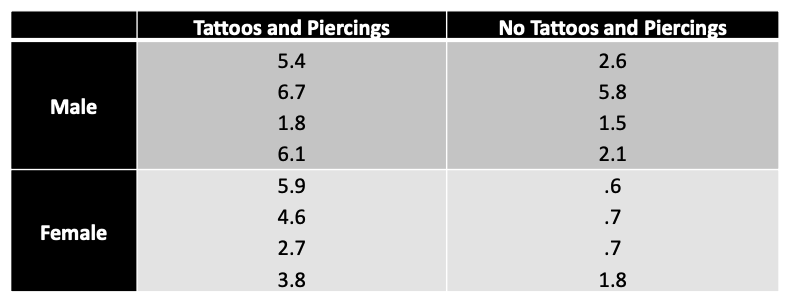
### Background
This research study is an adaptation of Gueguen (2012) described in Andy Field’s text. Specifically, the researchers hypothesized that **people with tattoos and piercings were more likely to engage in riskier behavior than those without tattoos and piercings**. In addition, the researcher wondered whether this difference varied, depending on whether a person was male or female.
Question: How many IVs? How many levels for each.
Answer: [2 IVs: (1) Whether or not having Tattos and Piercings (2) Male of Female. DV: Frequency of risk behaviors]{.mohu}
### Data screening
:::
## Step 1: Data importing
Either you can import a CSV file, or manually import the data points (for small samples).
Imagine you have a data with N = 16.
```{r}
tatto_piercing = rep(c(TRUE, FALSE), each = 8)
gender = rep(c("Male", "Female", "Male", "Female"), each = 4)
outcome = c(5.4, 6.7, 1.8, 6.1, 5.9, 4.6, 2.7, 3.8,
            2.6, 5.8, 1.5, 2.1, .6, .7, .7, 1.8)

dat <- data.frame(
  tatto_piercing = tatto_piercing,
  gender = gender,
  outcome = outcome
)
dat
```
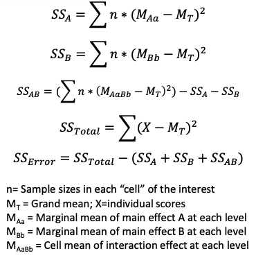
## Step 2: Sum of Squares of main effects
$$
SS_A = \sum n_a (M_{Aa} - M_T)^2
$$
- $M_{Aa}$ marginal mean of main effect A at each level
- $n_a$: sample size for factor A at each level
- $M_T$: grand mean of outcome
------------------------------------------------------------------------
### Obtain sum of square of tatto piercing
```{r}
#| include: false
summary(aov(data = dat, formula = outcome ~ gender * tatto_piercing))
```
#### Manual way
```{r}
M_A_table <-  dat |>
  group_by(tatto_piercing) |>
  summarise(
    N = n(),
    Mean = mean(outcome)
  )
M_T = mean(dat$outcome)
M_A_table
```
```{r}
M_A_table$N[1] * (M_A_table$Mean[1] - M_T)^2 +
  M_A_table$N[2] * (M_A_table$Mean[2] - M_T)^2
```
or
```{r}
sum(M_A_table$N * (M_A_table$Mean - M_T)^2)
```
------------------------------------------------------------------------
### Your turn: Obtain sum of squares of gender
```{webr-r}
#| context: setup
tatto_piercing = rep(c(TRUE, FALSE), each = 8)
gender = rep(c("Male", "Female", "Male", "Female"), each = 4)
outcome = c(5.4, 6.7, 1.8, 6.1, 5.9, 4.6, 2.7, 3.8,
2.6, 5.8, 1.5, 2.1, .6, .7, .7, 1.8)
dat <- data.frame(
tatto_piercing = tatto_piercing,
gender = gender,
outcome = outcome
)
dat
```
::: panel-tabset
### Exercise
`dat` object has already been loaded into R. Please, calculate the gender's sum of squares:
```{webr-r}
M_B_table <- dat |>
group_by(____) |>
summarise(
N = n(),
Mean = mean(___)
)
M_T = mean(____) ## grand mean
M_B_table
## Formula for Sum of squares of Gender
___[1] * (____[1] - ___)^2 +
___[2] * (____[2] - ____)^2
```
### Answer
```{webr-r}
M_B_table <- dat |>
group_by(gender) |>
summarise(
N = n(),
Mean = mean(outcome)
)
M_T = mean(dat$outcome) ## grand mean
M_B_table
M_B_table$N[1] * (M_B_table$Mean[1] - M_T)^2 +
M_B_table$N[2] * (M_B_table$Mean[2] - M_T)^2
```
:::
## Step 3: Sum of Squares of interaction effect
$$
SS_{AB} = (\sum n_{ab} (M_{AaBb} - M_T)^2) - SS_A - SS_B
$$

```{r}
cell_means <- dat |>
  group_by(tatto_piercing, gender) |>
  summarise(
    N = n(),
    Mean = mean(outcome)
  )
cell_means
```
------------------------------------------------------------------------
### Your turn
The data frame --- `cell_means` is already available to you.
```{webr-r}
#| context: setup
cell_means <- dat |>
group_by(tatto_piercing, gender) |>
summarise(
N = n(),
Mean = mean(outcome)
)
```
::: panel-tabset
### Exercise
Note: Sum of squares of interaction effects is the leftover of total sum of squares after removing SS of gender and SS of tutoring program.
$SS_{total} = \Sigma (N_{ab} * (M_{ab} - M_T))$
where $N_{ab}$ is the cell sample size for a-level of factor A and b-level of factor B.
$M_{ab}$ is the cell means of outcome; $M_T$ is the grand mean of outcome.
```{webr-r}
SS_gender <- 7.84
SS_TP <- 28.09
M_T <- 3.3
SS_total <- sum(____ * (____ - ___)^2)
SS_GxTP <- SS_total - ____ - ____
print(SS_GxTP)
```
### Answer
```{webr-r}
SS_gender <- 7.84
SS_TP <- 28.09
M_T <- 3.3
SS_total <- sum(____ * (____ - ___)^2)
SS_GxTP <- SS_total - ____ - ____
print(SS_GxTP)
sum(cell_means$N * (cell_means$Mean - M_T)^2) - SS_gender - SS_TP
```
:::
## Step 4: Calculate Degree of freedom and F-statistics
::: panel-tabset
### Your turn
```{webr-r}
#| context: setup
SS_gender <- 7.84
SS_TP <- 28.09
M_T <- 3.3
SS_GxTP <- sum(cell_means$N * (cell_means$Mean - M_T)^2) - SS_gender - SS_TP
SS_total <- sum((dat$outcome - mean(dat$outcome))^2)
SS_residual = SS_total - SS_gender - SS_TP - SS_GxTP
```
```{webr-r}
## Calculate total sum of square and residual SS
SS_total <- sum((dat$outcome - mean(dat$outcome))^2)
SS_residual = SS_total - SS_gender - SS_TP - SS_GxTP
df_gender = ___ # degree of freedom of factor gender
df_TP = ___ # degree of freedom of factor tutoring
df_GxTP = _____ # degree of freedom of interaction term gender x tutoring
df_residual = __ - __ - __ - __ - ___ # degree of freedom of residuals
F_gender = (___ / df_gender) / (SS_residual / df_residual)
F_TP = (___ / df_TP) / (SS_residual / df_residual)
F_GxTP = (___ / df_GxTP) / (SS_residual / df_residual)
F_gender; F_TP; F_GxTP # print out three F-statistics
```
### Answer
```{webr-r}
df_gender = 1
df_TP = 1
df_GxTP = 1*1
df_residual = 16 - 1 - 1 - 1 - 1*1
F_gender = (SS_gender / df_gender) / (SS_residual / df_residual)
F_TP = (SS_TP / df_TP) / (SS_residual / df_residual)
F_GxTP = (SS_GxTP / df_GxTP) / (SS_residual / df_residual)
F_gender; F_TP; F_GxTP # print out three F-statistics
#                       Df Sum Sq Mean Sq F value Pr(>F)
# gender                 1   7.84   7.840   2.942  0.112
# tatto_piercing         1  28.09  28.090  10.540  0.007 **
# gender:tatto_piercing  1   1.69   1.690   0.634  0.441
# Residuals             12  31.98   2.665
```
:::
## Interpretation
```
# Df Sum Sq Mean Sq F value Pr(>F)
# gender 1 7.84 7.840 2.942 0.112
# tatto_piercing 1 28.09 28.090 10.540 0.007 **
# gender:tatto_piercing 1 1.69 1.690 0.634 0.441
# Residuals 12 31.98 2.665
```
- Main Effect of Tattoo-Piercing: Reject the null → Ignoring the gender, there is a significant main effect of tattoo on risky behavior.
- Main Effect of Gender: Retain the null → Ignoring the tattoo, there is NO significant main effect of gender on risky behavior.
- Interaction: Retain the null → Under alpha=.05 level, because F-observed (F=0.63) does not exceed the critical value (F=4.75), we fail to reject the null that the effect of Factor A depends on Factor B. → “There is NO significant interaction between gender and tattoo on risky behavior.”
## Final discussion
In this example,
- The interaction effect shows several issues:
- Violation of independency assumption
- Violation of normality assumption in the condition of "Male" and "Tattoo=Yes"
- We can guess/think about one possibility that it might be cause by several reasons. (e.g., too small sample sizes, not randomized assignments of the samples, not a significant interaction effect, etc.)
- From the two-way ANOVA results, we found that the interaction effect is not significant.
- Thus, in this case, it is more reasonable to conduct
1. one-way ANOVA for "Group" variable, and
2. one-way ANOVA for "Gender" variable, separately.
- For each of one-way ANOVAs, we should check the assumptions, conduct one-way ANOVA, and post-hoc test separately as well.
## Exercise: Two-Way ANOVA with Significant Interaction
::: panel-tabset
### Background
A researcher is investigating the effect of **learning environment** (Online vs. In-Person) and **feedback type** (Immediate vs. Delayed) on student test scores. The researcher hypothesizes that:
1. Students in in-person classes will perform better than online students
2. Immediate feedback will lead to better performance than delayed feedback
3. **The benefit of immediate feedback will be stronger in online environments** (interaction effect)
The study randomly assigned 20 students to one of four conditions:
- Online + Immediate Feedback (n=5)
- Online + Delayed Feedback (n=5)
- In-Person + Immediate Feedback (n=5)
- In-Person + Delayed Feedback (n=5)
**Your Task**: Calculate the sum of squares for both main effects and the interaction effect manually, then compute F-statistics.
### View Data Summary
```{webr-r}
#| context: setup
set.seed(456)
# Create data with significant interaction
learning_env <- rep(c("Online", "In-Person"), each = 10)
feedback_type <- rep(c("Immediate", "Delayed"), times = 10)
# Test scores - designed to show interaction
# Online + Immediate: high scores (mean ~85)
# Online + Delayed: low scores (mean ~70)
# In-Person + Immediate: moderate scores (mean ~78)
# In-Person + Delayed: moderate-high scores (mean ~82)
test_scores <- c(
# Online + Immediate
87, 83, 88, 86, 81,
# Online + Delayed
68, 72, 71, 69, 70,
# In-Person + Immediate
79, 77, 80, 76, 78,
# In-Person + Delayed
84, 81, 83, 80, 82
)
exercise_data <- data.frame(
Learning_Env = factor(learning_env, levels = c("Online", "In-Person")),
Feedback = factor(feedback_type, levels = c("Immediate", "Delayed")),
Score = test_scores
)
# Display the data
exercise_data
```
```{webr-r}
# Cell means
cell_summary <- exercise_data |>
group_by(Learning_Env, Feedback) |>
summarise(
N = n(),
Mean = mean(Score),
SD = sd(Score)
)
print(cell_summary)
# Marginal means for Learning Environment
marginal_env <- exercise_data |>
group_by(Learning_Env) |>
summarise(
N = n(),
Mean = mean(Score)
)
print(marginal_env)
# Marginal means for Feedback Type
marginal_feedback <- exercise_data |>
group_by(Feedback) |>
summarise(
N = n(),
Mean = mean(Score)
)
print(marginal_feedback)
# Grand mean
grand_mean <- mean(exercise_data$Score)
print(paste("Grand Mean:", round(grand_mean, 2)))
```
### Step 1: Calculate SS for Learning Environment
**Formula**: $SS_A = \sum n_a (M_{Aa} - M_T)^2$
where: - $M_{Aa}$ = marginal mean of Learning Environment at each level - $n_a$ = sample size for each level of Learning Environment - $M_T$ = grand mean
```{webr-r}
# Calculate marginal means for Learning Environment
M_Env_table <- exercise_data |>
group_by(Learning_Env) |>
summarise(
N = n(),
Mean = mean(Score)
)
M_T <- mean(exercise_data$Score) # Grand mean
# Calculate SS for Learning Environment
SS_Env <- ___[1] * (___[1] - ___)^2 +
___[2] * (___[2] - ___)^2
print(paste("SS for Learning Environment:", round(SS_Env, 2)))
```
### Step 2: Calculate SS for Feedback Type
**Formula**: $SS_B = \sum n_b (M_{Bb} - M_T)^2$
```{webr-r}
# Calculate marginal means for Feedback Type
M_Feedback_table <- exercise_data |>
group_by(____) |>
summarise(
N = n(),
Mean = mean(____)
)
M_T <- mean(____) # Grand mean
# Calculate SS for Feedback Type
SS_Feedback <- ____$N[1] * (____$Mean[1] - ____)^2 +
____$N[2] * (____$Mean[2] - ____)^2
print(paste("SS for Feedback Type:", round(SS_Feedback, 2)))
```
### Step 3: Calculate SS for Interaction
**Formula**: $SS_{AB} = (\sum n_{ab} (M_{AaBb} - M_T)^2) - SS_A - SS_B$
```{webr-r}
# Calculate cell means
cell_means_table <- exercise_data |>
group_by(____, ____) |>
summarise(
N = n(),
Mean = mean(____)
)
print(cell_means_table)
# Calculate total SS from cells
SS_total_cells <- sum(____$N * (____$Mean - ____)^2)
# Calculate interaction SS
SS_Interaction <- ____ - ____ - ____
print(paste("SS for Interaction:", round(SS_Interaction, 2)))
```
### Step 4: Calculate F-statistics
```{webr-r}
# Calculate residual SS
SS_total <- sum((exercise_data$Score - mean(exercise_data$Score))^2)
SS_residual <- ____ - ____ - ____ - ____
# Calculate degrees of freedom
df_Env <- ____ # levels - 1
df_Feedback <- ____ # levels - 1
df_Interaction <- ____ * ____ # df_Env * df_Feedback
df_residual <- 20 - ____ - ____ - ____ - ____
# Calculate F-statistics
F_Env <- (SS_Env / df_Env) / (____ / ____)
F_Feedback <- (____ / ____) / (SS_residual / df_residual)
F_Interaction <- (____ / ____) / (____ / ____)
print(paste("F for Learning Environment:", round(F_Env, 3)))
print(paste("F for Feedback Type:", round(F_Feedback, 3)))
print(paste("F for Interaction:", round(F_Interaction, 3)))
```
### Answer - Step 1
```{webr-r}
# Calculate marginal means for Learning Environment
M_Env_table <- exercise_data |>
group_by(Learning_Env) |>
summarise(
N = n(),
Mean = mean(Score)
)
M_T <- mean(exercise_data$Score) # Grand mean
# Calculate SS for Learning Environment
SS_Env <- M_Env_table$N[1] * (M_Env_table$Mean[1] - M_T)^2 +
M_Env_table$N[2] * (M_Env_table$Mean[2] - M_T)^2
print(paste("SS for Learning Environment:", round(SS_Env, 2)))
```
### Answer - Step 2
```{webr-r}
# Calculate marginal means for Feedback Type
M_Feedback_table <- exercise_data |>
group_by(Feedback) |>
summarise(
N = n(),
Mean = mean(Score)
)
M_T <- mean(exercise_data$Score) # Grand mean
# Calculate SS for Feedback Type
SS_Feedback <- M_Feedback_table$N[1] * (M_Feedback_table$Mean[1] - M_T)^2 +
M_Feedback_table$N[2] * (M_Feedback_table$Mean[2] - M_T)^2
print(paste("SS for Feedback Type:", round(SS_Feedback, 2)))
```
### Answer - Step 3
```{webr-r}
# Calculate cell means
cell_means_table <- exercise_data |>
group_by(Learning_Env, Feedback) |>
summarise(
N = n(),
Mean = mean(Score)
)
print(cell_means_table)
# Calculate total SS from cells
SS_total_cells <- sum(cell_means_table$N * (cell_means_table$Mean - M_T)^2)
# Calculate interaction SS
SS_Interaction <- SS_total_cells - SS_Env - SS_Feedback
print(paste("SS for Interaction:", round(SS_Interaction, 2)))
```
### Answer - Step 4
```{webr-r}
# Calculate residual SS
SS_total <- sum((exercise_data$Score - mean(exercise_data$Score))^2)
SS_residual <- SS_total - SS_Env - SS_Feedback - SS_Interaction
# Calculate degrees of freedom
df_Env <- 1 # 2 levels - 1
df_Feedback <- 1 # 2 levels - 1
df_Interaction <- 1 * 1 # df_Env * df_Feedback
df_residual <- 20 - 1 - 1 - 1 - 1
# Calculate F-statistics
F_Env <- (SS_Env / df_Env) / (SS_residual / df_residual)
F_Feedback <- (SS_Feedback / df_Feedback) / (SS_residual / df_residual)
F_Interaction <- (SS_Interaction / df_Interaction) / (SS_residual / df_residual)
print(paste("F for Learning Environment:", round(F_Env, 3)))
print(paste("F for Feedback Type:", round(F_Feedback, 3)))
print(paste("F for Interaction:", round(F_Interaction, 3)))
# Calculate p-values
p_Env <- pf(F_Env, df_Env, df_residual, lower.tail = FALSE)
p_Feedback <- pf(F_Feedback, df_Feedback, df_residual, lower.tail = FALSE)
p_Interaction <- pf(F_Interaction, df_Interaction, df_residual, lower.tail = FALSE)
print(paste("p-value for Learning Environment:", round(p_Env, 4)))
print(paste("p-value for Feedback Type:", round(p_Feedback, 4)))
print(paste("p-value for Interaction:", round(p_Interaction, 4)))
```
### Verify with R's aov()
```{webr-r}
# Verify your calculations with R's built-in ANOVA
fit <- aov(Score ~ Learning_Env * Feedback, data = exercise_data)
summary(fit)
```
### Interpretation
```{webr-r}
# Visualize the interaction
library(ggplot2)
interaction_plot <- exercise_data |>
group_by(Learning_Env, Feedback) |>
summarise(Mean_Score = mean(Score)) |>
ggplot(aes(x = Learning_Env, y = Mean_Score, color = Feedback, group = Feedback)) +
geom_point(size = 4) +
geom_line(linewidth = 1.2) +
labs(title = "Interaction Plot: Learning Environment × Feedback Type",
x = "Learning Environment",
y = "Mean Test Score",
color = "Feedback Type") +
theme_minimal() +
theme(text = element_text(size = 12))
print(interaction_plot)
```
**Key Findings:**
1. **Main Effect of Learning Environment**: The effect depends on whether it's significant (check your F-statistic and p-value)
2. **Main Effect of Feedback Type**: The effect depends on whether it's significant (check your F-statistic and p-value)
3. **Interaction Effect**: **This should be significant!** The interaction plot shows that:
- In **Online** environments, Immediate feedback leads to MUCH higher scores than Delayed feedback
- In **In-Person** environments, the difference between Immediate and Delayed feedback is smaller (and reversed!)
- This crossing pattern indicates a strong interaction: the effect of feedback type depends on the learning environment
:::
## Lecture Summary: Key Takeaways
::: callout-tip
### 1. Conceptual Understanding
**Two-way ANOVA allows us to:**
- Examine the effects of **two independent variables** simultaneously
- Test for **three distinct effects**: Main effect A, Main effect B, and Interaction A×B
- Investigate whether the effect of one factor **depends on** the level of another factor (interaction)
- Achieve greater statistical power and efficiency compared to multiple one-way ANOVAs
**Main Effects vs. Interaction:**
- **Main Effect**: The average effect of one factor, ignoring (collapsing across) the other factor
- **Interaction Effect**: When the effect of one factor changes depending on the level of the other factor
- Look for **non-parallel lines** in interaction plots
- **Crossing lines** indicate strong interactions
- When interaction is significant, main effects may be misleading!
:::
------------------------------------------------------------------------
::: callout-important
### 2. Statistical Calculations
**Partitioning Variance in Two-Way ANOVA:**
$$
SS_{Total} = SS_A + SS_B + SS_{AB} + SS_{Residual}
$$
**Key Formulas:**
- Main Effect A: $SS_A = \sum n_a (M_{Aa} - M_T)^2$
- Main Effect B: $SS_B = \sum n_b (M_{Bb} - M_T)^2$
- Interaction: $SS_{AB} = (\sum n_{ab} (M_{AaBb} - M_T)^2) - SS_A - SS_B$
**F-statistics:**
$$
F = \frac{MS_{effect}}{MS_{residual}} = \frac{SS_{effect}/df_{effect}}{SS_{residual}/df_{residual}}
$$
**Degrees of Freedom:**
- $df_A = k_A - 1$ (number of levels of Factor A minus 1)
- $df_B = k_B - 1$ (number of levels of Factor B minus 1)
- $df_{AB} = df_A \times df_B$ (interaction df)
- $df_{residual} = N - 1 - df_A - df_B - df_{AB}$
:::
------------------------------------------------------------------------
::: callout-note
### 3. Practical Considerations
**Assumptions for Two-Way ANOVA:**
1. **Independence**: Observations must be independent (most critical!)
2. **Normality**: DV should be normally distributed within each cell
3. **Homogeneity of Variance**: Equal variances across all cells (Levene's test)
**Robustness:**
- F-test is fairly robust to normality violations with large N and equal cell sizes
- Recommend at least **15 participants per cell**
- Use Welch or Brown-Forsythe tests if variances are unequal
- **Never** compromise on independence assumption
**Type I, II, III Sum of Squares:**
- **Type I**: Sequential (order matters) - appropriate for nested/blocking designs
- **Type II**: Each main effect adjusted for other main effects - good for model building
- **Type III**: Each effect adjusted for all others - **recommended for factorial designs** with balanced data
- With **balanced designs** (equal cell sizes), all three types give identical results!
:::
------------------------------------------------------------------------
::: callout-warning
### 4. Interpretation Guidelines
**When Interaction is Significant:**
- Interpret interaction **first** before discussing main effects
- Main effects may be misleading or uninterpretable when interaction is present
- Focus on **simple effects**: the effect of one factor at each level of the other
- Use interaction plots to visualize and explain the pattern
**When Interaction is NOT Significant:**
- Proceed to interpret main effects
- If main effect is significant with \>2 levels, conduct **post-hoc tests** (e.g., Tukey HSD)
- Report effect sizes (partial η²) alongside p-values
**Reporting Results:**
Include in your report:
1. Descriptive statistics (means, SDs) for all cells
2. ANOVA table with F-values, df, and p-values
3. Effect sizes
4. Interaction plot (even if not significant)
5. Post-hoc tests if needed
6. Assumption checks
:::
------------------------------------------------------------------------
::: callout-tip
### 5. Common Pitfalls to Avoid
1. **Don't ignore significant interactions!** Main effects alone don't tell the whole story
2. **Don't forget assumption checks** - especially for small samples
3. **Don't confuse interaction with correlation** - they are different concepts
4. **Don't over-interpret non-significant results** - absence of evidence ≠ evidence of absence
5. **Don't use multiple one-way ANOVAs instead of two-way** - you'll miss interactions and inflate Type I error
6. **Don't forget to report effect sizes** - statistical significance ≠ practical significance
:::
------------------------------------------------------------------------
::: callout-important
### 6. Next Steps in Your Learning
**Extending Two-Way ANOVA:**
- **Three-way ANOVA**: Adding a third factor (exponentially more complex!)
- **Mixed ANOVA**: Combining between-subjects and within-subjects factors
- **ANCOVA**: Adding continuous covariates to control for confounding variables
- **MANOVA**: Multiple dependent variables simultaneously
- **Repeated Measures ANOVA**: Same subjects measured multiple times
**When to Use Two-Way ANOVA:**
✓ Two categorical independent variables (factors) ✓ One continuous dependent variable ✓ Independent observations (between-subjects design) ✓ Interest in both main effects and interaction ✓ Adequate sample size (≥15 per cell recommended)
**Alternatives to Consider:**
- **Regression with interactions**: More flexible, can handle continuous IVs
- **Mixed-effects models**: Better for unbalanced designs or nested data
- **Non-parametric tests**: When assumptions are severely violated (e.g., Aligned Rank Transform ANOVA)
:::
## Fin
**Thank you for your attention!**