Lecture 12: ANCOVA

Overview of Lecture 12

1. What is ANCOVA?
2. Why use ANCOVA?
3. How to use ANCOVA (e.g., assumptions, hypothesis setup)?
4. Potential issues of using ANCOVA.

1 Introduction

1.1 Introduction: Overview of Other Designs

• The ANOVA designs we have been talking about use experimental control (e.g., our research design) in order to reduce error variance.
  • ✔ Example: In the one-way ANOVA tutoring example, we posited that there might be another factor explaining math scores beyond the tutoring program (factor A).
  • ✔ Thus, we also looked at school type (factor B) to help reduce the error variance.
• Other examples to reduce error variance:
  • ✔ Blocking (analyzing blocks of experimental units – levels of IVs)
  • ✔ Between-subjects design (i.e., N-way ANOVA)
  • ✔ Within-subjects design (i.e., repeated measures)

1.2 Introduction: ANCOVA

ANOVA is Analysis of Variance

ANCOVA is Analysis of Covariance

• Today we focus on statistical control to reduce error variance.

• Statistical control is used when we know a subject’s score on an additional variable.

  • When we discussed blocking designs, the control variable was categorical (e.g., school, class).
  • But for ANCOVA, it is a continuous covariate!
    • e.g., students’ academic motivation, engagement, baseline math proficiency.

• What is “covariate”?

  • A covariate is an observed predictor not of primary interest, included to explain additional variance in the dependent variable.
  • In ANCOVA, covariates are modeled linearly and are assumed to be measured prior to or independent of treatment assignment.
  • Including covariates reduces residual error and adjusts group means, improving precision when assumptions hold (e.g., no treatment–covariate interaction, reliable measurement).
  • Example (one‑way ANCOVA): E[Y | Group, X] = α + τ_Group + βX, where X is the covariate, τ_Group are group effects, and β is the common slope.

• ANCOVA by definition is a general linear model that includes both:

  • ANOVA (categorical) predictors
  • Regression (continuous) predictors

1.3 ANCOVA: Example

• We are interested in

  • Comparing the method of instruction on students’ mathematical problem‑solving performance, as measured by a test score.

    • The test is composed of word problems that are each presented in a few sentences.
      • Ex: “Joe buys 60 cantaloupes and sells 5. He then gives away 4…”
      • DV = number of problems correctly answered in an hour.
      • IV = method of instruction (three levels)

• One-way, independent ANOVA: If the omnibus F is significant, we conclude that the instructional methods differ in the mean number of correctly answered problems.

• But, performance on math word problems may be affected by factors beyond instructional method and math ability.

  • To name a few: academic motivation scores, verbal proficiency scores, hunger ratings, previous years’ math grades…

• The DV score results from instructional method + the other factors we just listed.

  • We really want to ask:

    To what extent would we have observed instructional‑method differences in math scores if the groups had been equivalent in motivation (or verbal proficiency)?

1.4 ANCOVA definition

• ANCOVA is one way to investigate the group (treatment) effect controlling for some relevant covariates.
• Incorporates information on additional variables (e.g., motivation) directly into the model.
  • To estimate differences in math word‑problem performance as if the groups were equivalent in baseline motivation.
• When comparing groups, we claim that people vary in their scores on the DV for a variety of reasons:
  • Treatment Effects (i.e., group differences) - Ex: Instructional Method
  • Individual Differences - Ex: Individuals vary in their motivation to do well on the math test
  • Measurement Error - Ex: The math assessment is unreliable
  • These two sources (Individual differences and measurement error) contribute to:
    • Experimental Error
    • (both of these go into $SS_{\text{Error}}$)

1.5 ANCOVA Advantage

• Reduces Error Variance
  • By explaining some of the unexplained variance ($SS_{\text{error}}$), the error variance in the model can be reduced.
  • Think of the pie charts below!
• Greater Experimental Control
  • By controlling known extraneous variables, we gain greater insight into the effect of the predictor (IV) variable(s).

---

1.6 What covariate can be added?

• Including a covariate adjusts the groups’ means as if they were equivalent on the covariate.

• The analyses addressed different research questions!

  • Ex. Ignoring the impact of height
    ➔ $H_0\!: \mu_A = \mu_B = \mu_C$
  • Considering height (ANCOVA): adjusted means
    ➔ $H_0\!: \text{Adj}_{\mu_A} = \text{Adj}_{\mu_B} = \text{Adj}_{\mu_C}$

• If there is no random assignment to treatments, use ANCOVA with caution.
  • Pre‑existing differences may render the “as if equivalent” interpretation untenable.

1.7 ANCOVA: Backrgound of Example Case

• Consider a scenario in which a school principal wants to evaluate the effectiveness of teaching methods in math courses.
• The principal would like to gauge the effectiveness of the following three types of instruction:
  • Type 1: Lecture-only,
  • Type 2: Lecture + hands-on activities,
  • Type 3: Self-paced instruction
• The principal randomly assigned 200 students to one of the three instructional methods and measured performance on an end‑of‑semester achievement test (out of 100 points).
• One researcher suggested that the principal also want to statistically control for students’ ability (covariate):

Each student also completed a math pre‑test (an indicator of baseline ability), so the principal included pre‑test scores as the covariate.

1.8 ANCOVA: Example Data

In this example, we will simulate data for 200 students who were randomly assigned to one of three teaching methods.

The pre-test scores will be used as a covariate in the ANCOVA analysis.

The post-test scores will be generated based on the pre-test scores and the teaching method.

student_id	method	pretest	posttest
1	lecture	68.9	70.9
2	hands-on	66.1	62.8
3	lecture	61.6	53.5
4	self-paced	72.5	85.8
5	hands-on	64.9	73.1

Evaluating hidden code cell...

1

2

3

head(df)

table(df$method)

cor(df$pretest, df$posttest)

2 ANCOVA: Assumption Check

2.1 ANCOVA: Assumption Check I

Assumption Check in ANCOVA:

➤ The three usual ANOVA assumptions apply:

• Independency
• Normality (within-group; for each group)
• Equality of variance (homogeneity of variance)

➤ Three additional data considerations:

• Linear relationship between the covariate & DV
• Homogeneity of Regression Slope
• Covariate is measured without error

2.2 ANCOVA: Assumption Check II

• Assumption Check in ANCOVA:

1. Linear relationship between the covariate & DV:

---

By looking over the plot, we can find that there is a general linear relationship (i.e., straight line) between the covariate (pretest) and the DV (mathtest).

# Plot
ggplot(df, aes(x = pretest, y = posttest)) +
  geom_point(color = "blue", alpha = 0.6) +
  geom_smooth(method = "lm", color = "steelblue", se = FALSE) +
  theme_minimal(base_size = 14) +
  labs(x = "pretest", y = "mathtest") +
  theme(legend.position = "bottom") +
  guides(color = guide_legend(title = NULL))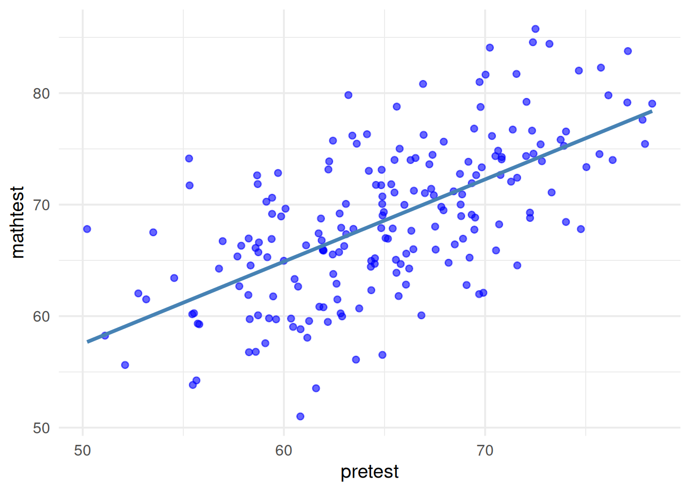

2.3 ANCOVA: Assumption Check III

• Assumption Check in ANCOVA:

2. Homogeneity of Regression Slope:

• The relationship between each covariate and the DV should be the same for each level of the IV.
  • Conceptually, this is the interaction between the IV and the covariate.
  • We don’t want this in ANCOVA!
  • This assumption limits the applicability of ANCOVA

---

import matplotlib.pyplot as plt
import numpy as np

# Generate x values (covariate)
x = np.linspace(0, 10, 100)

# Homogeneous regression slopes
y1_homo = 1.0 * x + 2
y2_homo = 1.0 * x + 4
y3_homo = 1.0 * x + 6

# Heterogeneous regression slopes
y1_hetero = -0.1 * x + 6
y2_hetero = 1.2 * x + 1
y3_hetero = 0.9 * x + 3

# Create the figure with two subplots
fig, axs = plt.subplots(1, 2, figsize=(12, 5), sharey=True)

# Plot for homogeneous regression slopes
axs[0].plot(x, y1_homo, label="Group 1")
axs[0].plot(x, y2_homo, label="Group 2")
axs[0].plot(x, y3_homo, label="Group 3")
axs[0].set_title("(a) Homogeneity of regression (slopes)")
axs[0].set_xlabel("Covariate (X)")
axs[0].set_ylabel("DV (Y)")
axs[0].legend()

# Plot for heterogeneous regression slopes
axs[1].plot(x, y1_hetero, label="Group 1")
axs[1].plot(x, y2_hetero, label="Group 2")
axs[1].plot(x, y3_hetero, label="Group 3")
axs[1].set_title("(b) Heterogeneity of regression (slopes)")
axs[1].set_xlabel("Covariate (X)")
axs[1].legend()

plt.tight_layout()
plt.show()

2.4 ANCOVA: Assumption Check IV

• Assumption Check in ANCOVA:

2. Homogeneity of Regression Slope:

➤ This is equivalent to saying that the relationship between the DV and the covariate must be the same for each cell (i.e., group).

• The slope value – b – that we use to make the adjustment is the same

➤ Consequences depend on whether cells have equal sample sizes and whether a true experiment

• With equal sample sizes in a true experiment, ANCOVA is relatively robust to modest violations of this assumption.
• With unequal sample sizes (or in quasi‑experimental designs), the adjusted means may be materially biased.

2.5 ANCOVA: Assumption Check V

• Assumption Check in ANCOVA:

2. Homogeneity of Regression Slope:

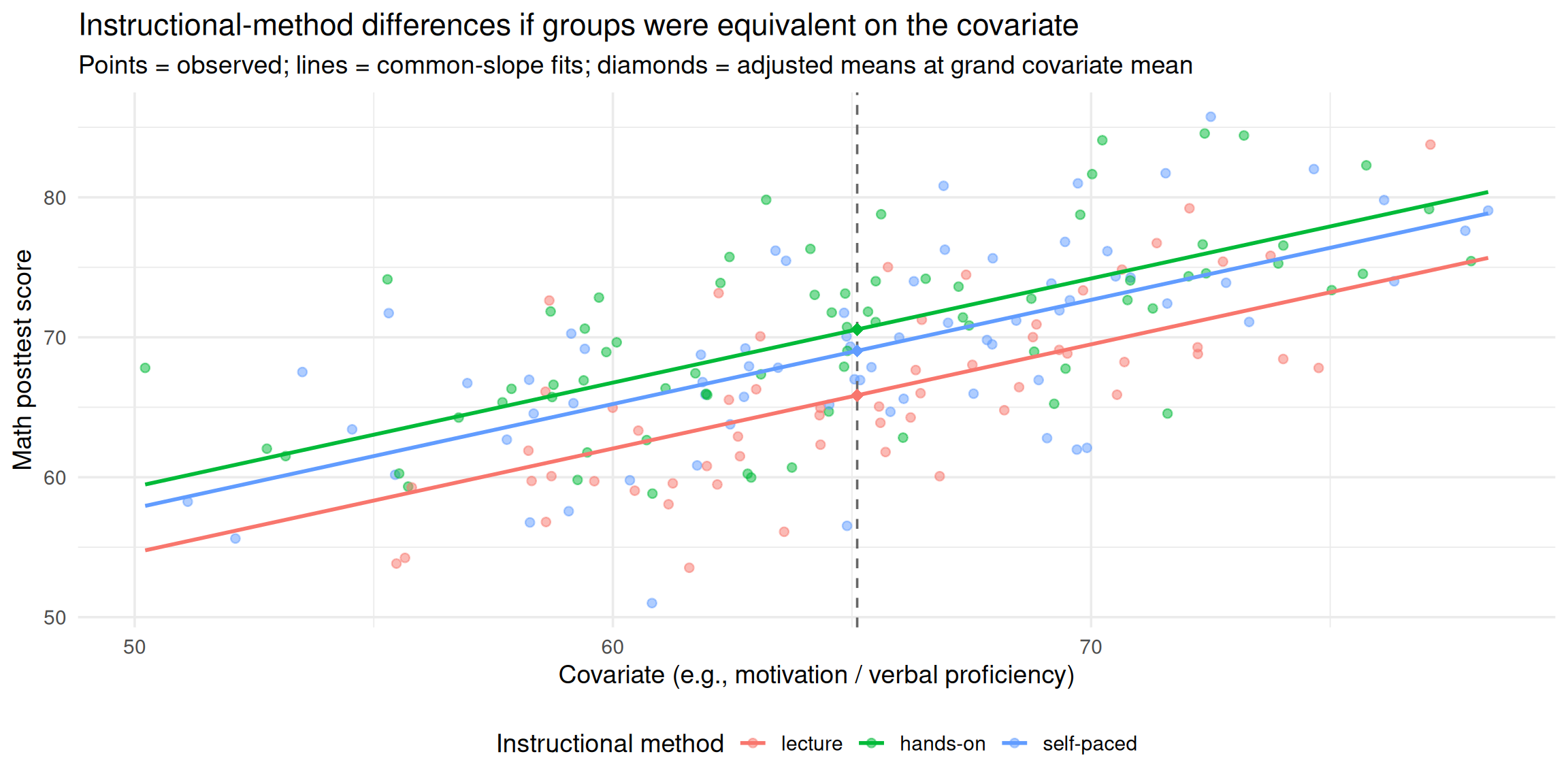
When we visually inspect the three regression slopes (covariate predicting the DV), the relationships appear approximately equal.

# Plot
ggplot(df, aes(x = pretest, y = posttest, color = method)) +
  geom_point(alpha = 0.6) +
  geom_smooth(method = "lm", se = FALSE) +
  scale_color_manual(values = c("steelblue", "tomato", "seagreen4")) +
  theme_minimal(base_size = 14) +
  labs(x = "pretest", y = "mathtest") +
  theme(legend.position = "bottom") +
  guides(color = guide_legend(title = NULL))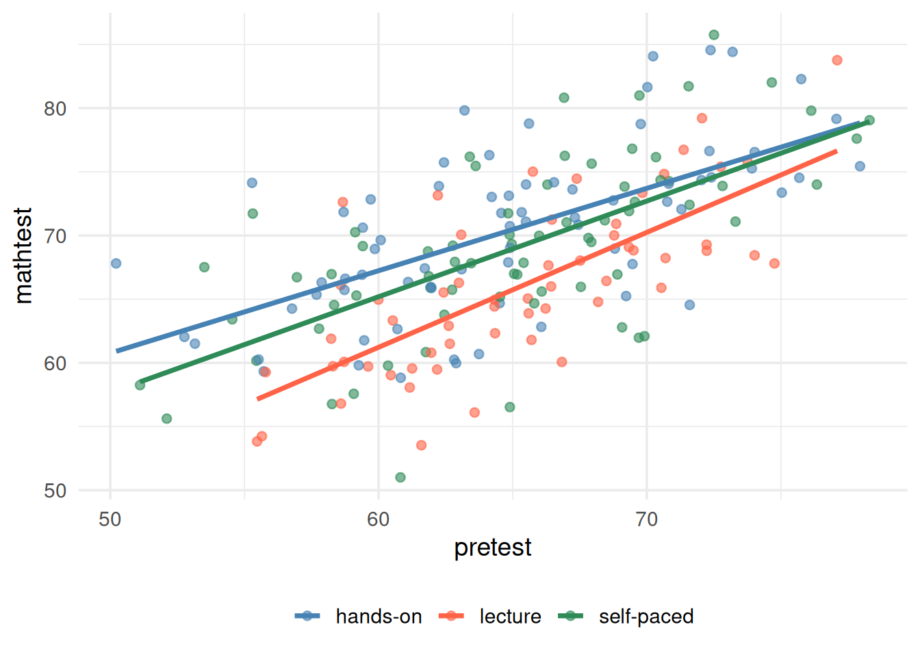

2.6 ANCOVA: Assumption Check VI

• Assumption Check in ANCOVA:

2. Homogeneity of Regression Slope:

➤ Formal approach to checking homogeneity of regression slopes:

1. Run the model with the interaction term included to make sure it is negligible (a.k.a., not significant) → this is not the ANCOVA yet!

$SS_{total} = SS_{IV} + SS_{COV} + \color{red}{SS_{IV*COV}} + SS_{within}$

2. If negligible (i.e., not significant), re‑run the ANCOVA without the interaction term to obtain the final estimates to interpret → this is the ANCOVA model.

$SS_{total} = SS_{IV} + SS_{COV} + SS_{within}$

2.7 ANCOVA: Assumption Check VII

2. Homogeneity of Regression Slope: ➤ The formal/general method of checking homogeneity of regression slope:

3. Run the model with the interaction term included to make sure it is negligible (a.k.a., not significant) → this is not the ANCOVA yet!

library(gt)
library(tidyverse)
res <- anova(lm(posttest~pretest*method, data=df))
res_tbl <- res |>
  as.data.frame() |>
  rownames_to_column("Coefficient")
res_gt_display <- gt(res_tbl) |>
  fmt_number(
    columns = `Sum Sq`:`Pr(>F)`,
    suffixing = TRUE,
    decimals = 3
  )
res_gt_display|>
  tab_style( # style for versicolor
    style = list(
      cell_fill(color = "royalblue"),
      cell_text(color = "red", weight = "bold")
    ),
    locations = cells_body(
        columns = colnames(res_tbl),
        rows = Coefficient == "pretest:method")
  )

Coefficient	Df	Sum Sq	Mean Sq	F value	Pr(>F)
pretest	1	3.774K	3.774K	150.059	0.000
method	2	726.111	363.055	14.436	0.000
pretest:method	2	66.190	33.095	1.316	0.271
Residuals	194	4.879K	25.148	NA	NA

2. IF negligible (a.k.a., not significant), re-run the ANCOVA without the interaction term to get the final values to interpret → this is the ANCOVA model.

res <- anova(lm(posttest~pretest+method, data=df))
res_tbl <- res |>
  as.data.frame() |>
  rownames_to_column("Coefficient")
res_gt_display <- gt(res_tbl) |>
  fmt_number(
    columns = `Sum Sq`:`Pr(>F)`,
    suffixing = TRUE,
    decimals = 3
  )
res_gt_display|>
  tab_style( # style for versicolor
    style = list(
      cell_fill(color = "royalblue"),
      cell_text(color = "red", weight = "bold")
    ),
    locations = cells_body(
        columns = colnames(res_tbl),
        rows = Coefficient == "method")
  )

Coefficient	Df	Sum Sq	Mean Sq	F value	Pr(>F)
pretest	1	3.774K	3.774K	149.576	0.000
method	2	726.111	363.055	14.390	0.000
Residuals	196	4.945K	25.230	NA	NA

2.8 ANCOVA: Assumption Check VIII

• Assumption Check in ANCOVA:

3. Covariate is measured without error:

➤ Reliability of Covariates

• ✓ Because covariates are used to linearly predict the DV, measurement error in the covariate is not modeled (unlike the DV).
• ✓ Thus, ANCOVA assumes covariates are measured without error.
  • ➔ You will cover reliability of measures in detail in measurement theory; here we simply note its importance.

➤ The reliability of covariate scores is crucial with ANCOVA

True Experimental Design	Quasi-Experimental Design
- Relationship between covariate and DV underestimated, resulting in less adjustment than is necessary	- Relationship between covariate and DV underestimated, resulting in less adjustment than is necessary
- Less powerful F test	- Group effects (IV) may be seriously biased

3 Hypothesis Test

3.1 ANCOVA: Hypothesis Test I

[Example] Step #1

• Research (alternative) hypothesis
  • $H_A$: Controlling for pretest, the adjusted means of math scores among three instructional groups will differ.
• Null hypothesis
  • $H_0$: Controlling for pre-test, there is no difference between the adjusted means of math scores among three instructional groups.
    $\Rightarrow H_0: \text{adjusted } \mu_{\text{lecture}} = \text{adjusted } \mu_{\text{hands-on}} = \text{adjusted } \mu_{\text{self-paced}}$

---

3.1.1 ANCOVA: Definition of Adjusted Means

• Adjusted cell means are the observed cell mean minus a weighted within-cell deviation of the covariate values from the covariate cell means.
  • When we do the adjustment, this is what happens:

$$\bar{Y}_{\text{adjusted}} = \bar{Y}_{\text{original}} - b (\bar{X}_{\text{cell}} - \bar{X}_{\text{grand}})$$

• b is the pooled slope for the simple regression of the DV on the covariate
  

• X is the covariate (cell mean and grand mean)
  

• Y is the dependent variable (adjusted and unadjusted cell means)

• If b is zero (relationship is zero) then there is no adjustment.

• The bigger b is (the stronger the covariate/DV relationship), the more of an adjustment.

➔ The farther a cell’s covariate mean is from the grand covariate mean (the larger the deviation), the greater the adjustment to its outcome mean.

---

3.1.2 ANCOVA: Formula of Adjusted Means

Based on the ANCOVA adjusted means formula:

$$\bar{Y}_{\text{adjusted}} = \bar{Y}_{\text{original}} - b (\bar{X}_{\text{cell}} - \bar{X}_{\text{grand}})$$ We can compute the adjusted means for each group using the following steps:

# Unadjusted means of posttest by group
unadjusted_means <- df %>%
  group_by(method) %>%
  summarise(posttest_mean = mean(posttest))

# Pretest means by group
pretest_means <- df %>%
  group_by(method) %>%
  summarise(pretest_mean = mean(pretest))

# Grand mean of pretest
grand_pretest_mean <- mean(df$pretest)

# Fit linear model to get pooled regression slope
model <- lm(posttest ~ pretest, data = df)

# Extract slope
pooled_slope <- coef(model)["pretest"]

# Combine into one table
results <- left_join(unadjusted_means, pretest_means, by = "method")

# Calculate adjusted means using the ANCOVA adjustment formula
results2 <- results |>
  mutate(grand_pretest_mean = grand_pretest_mean) |>
  mutate(pooled_slope = pooled_slope) |>
  mutate(adjusted_mean = posttest_mean - pooled_slope * (pretest_mean - grand_pretest_mean))

# View results
gt(results2) |>
  fmt_number(
    columns = posttest_mean:adjusted_mean
  )

method	posttest_mean	pretest_mean	grand_pretest_mean	pooled_slope	adjusted_mean
hands-on	70.41	64.90	65.11	0.74	70.56
lecture	65.96	65.25	65.11	0.74	65.86
self-paced	69.10	65.20	65.11	0.74	69.03

---

3.1.3 Visualization

Based on the adjusted means, pretest, and posttest means, we can visualize the results using a bar plot.

used_colors <- c("steelblue", "tomato", "seagreen4")
used_group_labels <- c("Pretest", "Posttest", "Adjusted")
results2 |>
  select(method, pretest_mean, posttest_mean, adjusted_mean) |>
  pivot_longer(ends_with("_mean"), names_to = "type", values_to = "Mean") |>
  mutate(type = factor(type, levels = paste0(c("pretest", "posttest", "adjusted"), "_mean"))) |>
  ggplot(aes(y = method, x = Mean)) +
  geom_col(aes(y = method, x = Mean, fill = type), position = position_dodge()) +
  geom_text(aes(x = Mean + 5, label = round(Mean, 2), color = type), position = position_dodge(width = .85)) +
  scale_color_manual(values = used_colors, labels = used_group_labels) +
  scale_fill_manual(values = used_colors, labels = used_group_labels) +
  labs(y = "", title = "Comparing Adjusted and Unadjusted Means") +
  theme_minimal() +
  theme(legend.position = "bottom")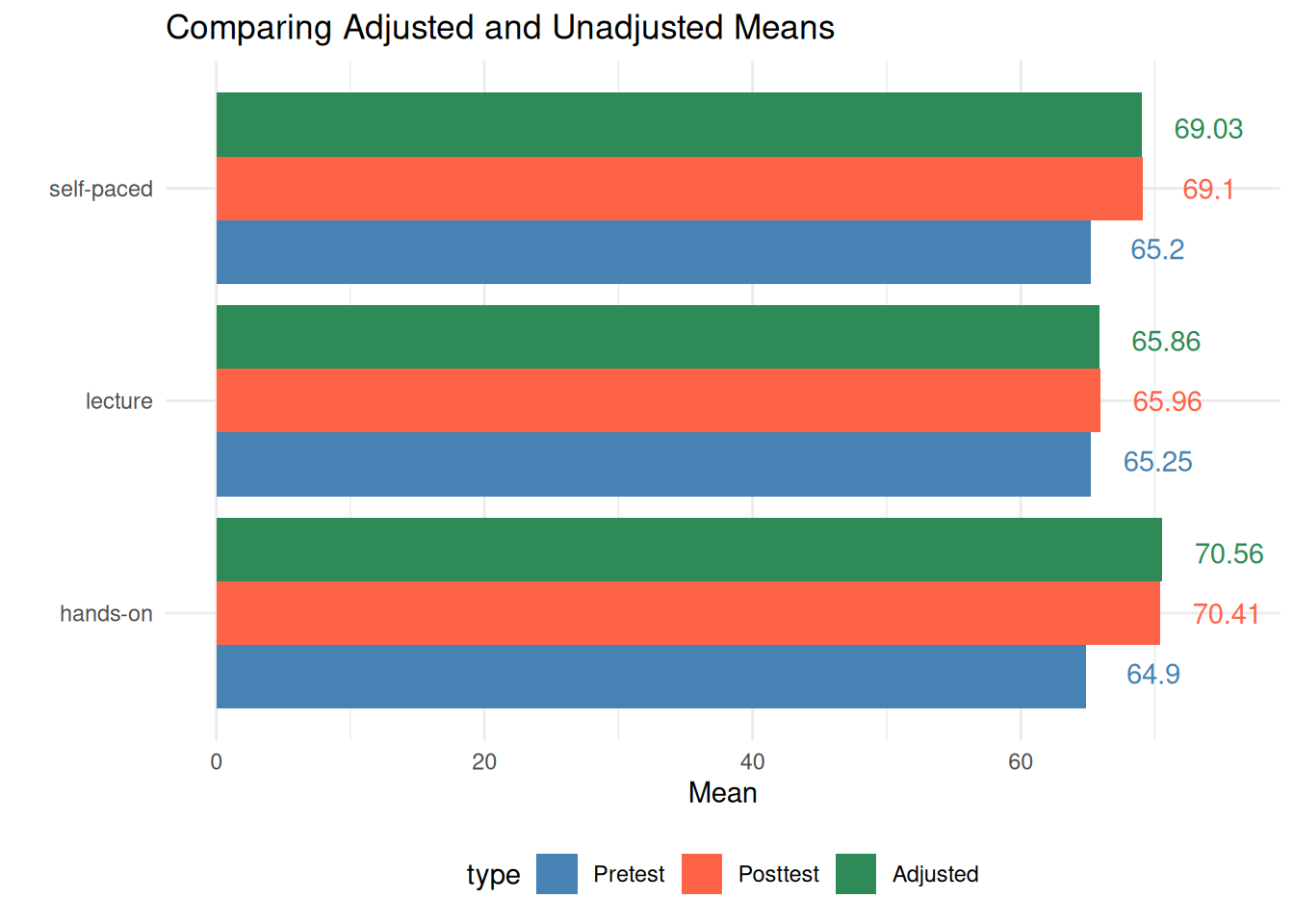

3.2 ANCOVA: Hypothesis Test II

• [Example] Step #2

• Recall: What distinguishes ANCOVA from other analyses?

• In addition to a grouping variable (IV), we have scores from some continuous measure (i.e., covariate) that is related to the DV

  • Preferably, we are in a randomized-control experimental situation — use caution when in a quasi-experimental situation! (because it does not consider random assignments of treatments/levels of IV)

• This is a situation in which we desire “statistical control” based upon the covariate.

  • In some scenarios it may not make sense to adjust the group means as if they were the same on the covariate.

• In ANCOVA:

  • IV: same as before — grouping/categorical variable with 2 or more levels
  • In addition to IV, we are adding a continuous covariate → this is NEW!
  • DV: same as before — continuous variable

3.3 ANCOVA: Hypothesis Test III

• [Example] Step #2

• Recall: Continuous covariate?

• ➤ Categorical variable

  • ✓ Contain a finite number of categories or distinct groups.

  • ✓ Might not have a logical order.

  • ✓ Examples: gender, material type, and payment method.

• ➤ Discrete variable

  • ✓ Numeric variables that have a countable number of values between any two values.

  • ✓ Examples: number of customer complaints, number of items correct on an assessment, attempts on GRE.

  • ✓ It is common practice to treat discrete variables as continuous, as long as there are a large number of levels (e.g., 1–100 not 1–4).

• ➤ Continuous variable

  • ✓ Numeric variables that have an infinite number of values between any two values.

  • ✓ Examples: length, weight, time to complete an exam.

• ➔ We often assume the DV for ANCOVA is continuous, but we can sometimes “get away” with discrete, ordered outcomes if there are enough categories.

3.4 ANCOVA: Hypothesis Test IV

• [Example] Step #2
• What if we have a categorical outcome?

➤ Not related to this course, but categorical outcomes are commonly analyzed: - ✓ Examples: pass/fail a fitness test; pass/fail an academic test; retention (yes/no); on-time graduation (yes/no); proficiency (below, meeting, advanced), etc.

➔ These are not continuous, so we cannot use them in ANOVA

➤ Instead: logistic regression (PROC LOGISTIC or PROC GLM!) - ✓ Logistic regression can include both categorical and continuous IVs (and their interactions)

# Load libraries
library(ggplot2)
library(dplyr)

# Simulate data
set.seed(123)
n <- 100
weight <- rnorm(n, 140, 20)
prob_obese <- 1 / (1 + exp(-(0.1 * weight -15)))  # logistic model
obese <- rbinom(n, size = 1, prob = prob_obese)

data <- data.frame(weight = weight, obese = obese)

# Linear model
lm_model <- lm(obese ~ weight, data = data)

# Logistic model
logit_model <- glm(obese ~ weight, data = data, family = "binomial")

# Prediction data
pred_data <- data.frame(weight = seq(min(weight), max(weight), length.out = 100))
pred_data$lm_pred <- predict(lm_model, newdata = pred_data)
pred_data$logit_pred <- predict(logit_model, newdata = pred_data, type = "response")

# Plot 1: Linear Regression
p1 <- ggplot(data, aes(x = weight, y = obese)) +
  geom_point(color = "red", size = 2) +
  geom_line(data = pred_data, aes(x = weight, y = lm_pred), color = "black") +
  labs(title = "Linear Regression", x = "weight", y = "Obesity (0/1)") +
  # ylim(0, 1.1) +
  theme_minimal()

# Plot 2: Logistic Regression
p2 <- ggplot(data, aes(x = weight, y = obese)) +
  geom_point(color = "red", size = 2) +
  geom_line(data = pred_data, aes(x = weight, y = logit_pred), color = "black") +
  labs(title = "Logistic Regression", x = "weight", y = "Predicted Probability") +
  # ylim(0, 1.1) +
  theme_minimal()

# Combine plots using patchwork
library(patchwork)
p1 + p2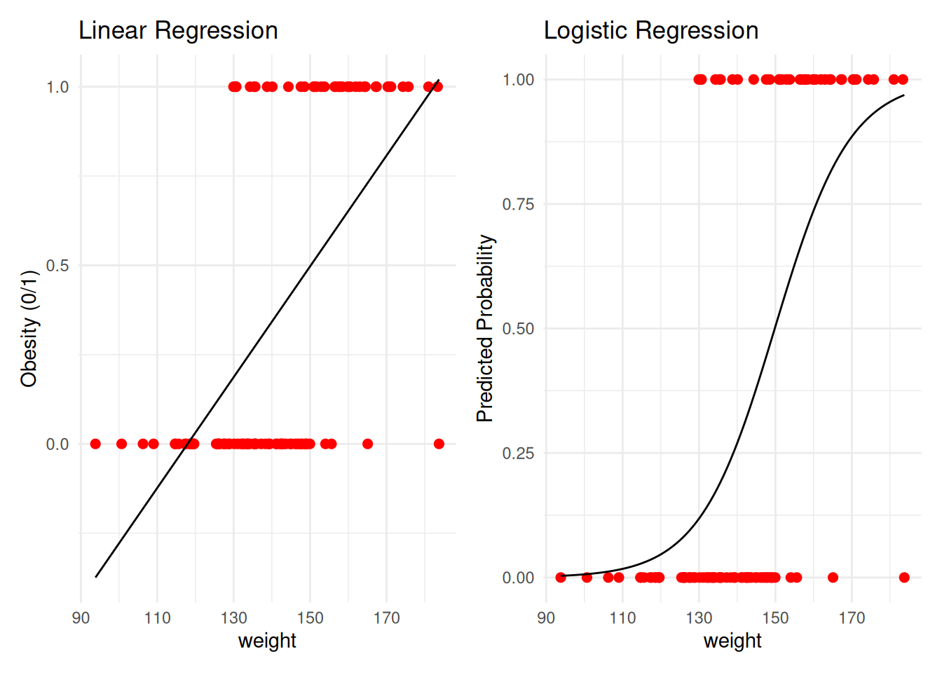

3.5 ANOVA: Degree of Freedom

• In addition to the traditional degrees of freedom for ANOVA, you lose one degree of freedom for each covariate.

• Degrees of Freedom → In our scenario, we have 1 IV with 3 groups and 1 covariate.

• The $df_{method}$ remains: k − 1, where k is the number of groups.

  • In our scenario, with 3 groups, the numerator df = 3 − 1 = 2

• The $df_{error}$ differs from ANOVA:

  • N − k − c, where k is the number of groups and c is the number of covariates.
  • In our scenario, if there are 200 students (N = 200), 3 groups, and 1 covariate (e.g., IQ), the df is
    200 − 3 − 1 = 196

• The $df_{covariate}$ is #covariates = 1

• With 200 students, 3 groups, and 1 covariate, the degrees of freedom for this analysis would be:

  • 2 (numerator) and 196 (denominator)

3.6 AFTER ANCOVA: Treatment Effect

• Now we need to follow-up to see where the differences lie.

• Planned contrasts and pairwise comparisons

  • based on the adjusted means and the error term after removing covariate variance
  • Can interpret the same, just be sure to note that it is the effect for the adjusted means
    (i.e., the means of DV after controlling for covariate)

• Post-hoc tests

  • Many post‑hoc procedures are not designed for ANCOVA; however, a limited selection is available (e.g., Bonferroni, Sidak). Avoid mislabeling Tukey’s HSD as “LSD.”

3.7 Problem: ANCOVA in Quasi-experimental Design I

	True Experimental Design	Quasi-Experimental Design
Assignment to treatment	The researcher randomly assigns subjects to control and treatment groups.	Some other, non-random method is used to assign subjects to groups.
Control over treatment	The researcher usually designs the treatment.	The researcher often does not have control over the treatment, but studies pre-existing groups.
Use of control groups	Requires the use of control and treatment groups.	Control groups are not required (although they are commonly used).

3.8 Problem: ANCOVA in Quasi-experimental Design II

• ANCOVA in true experiments is straightforward
  • It reduces error variance and increases power and is a great option if you have a good covariate and have met the ANCOVA assumptions.
• ANCOVA in quasi‑experimental designs is controversial and risky
  • Some people say you shouldn’t do it at all. Others say you just have to be careful not to over-interpret and to be sure to do replications.
• Accounting for Pre-Existing Group Differences:
  • ➤ If people are not randomly assigned to conditions, there may be differences in the DV across the groups before the experiment starts.
  • ➤ Some use ANCOVA to “account for pre‑existing differences” in quasi‑experimental designs; however:
    • ANCOVA equates groups on a particular covariate, but there is no guarantee that this is the only or most important dimension that the groups differ on.
    • Equating pre‑existing groups on one variable may accentuate differences on another.

3.9 Problem: ANCOVA in Quasi-experimental Design III

• What is the risk/concern with quasi-experimental design?

  ➤ For example, including a covariate adjusts the two groups’ means as if they were the same on that covariate.
  ➤ Therefore, the two analyses are addressing two different research questions!

  • Pre–post change analysis addresses $H_0\!: \mu_{\text{female}} = \mu_{\text{male}}$
  • ANCOVA addresses $H_0\!: \text{adjusted } \mu_{\text{female}} = \text{adjusted } \mu_{\text{male}}$

Biases the effect size of the IV	Values can’t be trusted
- Can remove real “effect variance” and attenuate the effect size	- Adjusted means are implausible values
- If other variables involved, can make it look like there is an effect when there isn’t	- Interaction and slope values could just apply to the cells observed, not the population

3.10 ANCOVA: Final Thoughts…

• Use of covariates does not guarantee that groups are “equivalent” —
  even after using multiple covariates, there still may be some confounding variables operating that you are unaware of.

• The best safeguard against confounding is random assignment to groups.

• Make sure that the covariate you are using is reliable!

Final Exercise: Psychology Scenario (ANCOVA)

• Scenario: Therapy effectiveness on anxiety reduction
• Outcome (continuous): post_anxiety
• IV (categorical, 3 levels): therapy (CBT, Mindfulness, Control)
• Covariate 1 (categorical): sex (Female/Male)
• Covariate 2 (continuous): baseline anxiety (pre_anxiety)

Starter Code

Evaluating hidden cell 1 out of 2

1

2

3

4

5

6

7

8

9

10

11

12

13

14

15

16

17

18

19

20

21

22

23

24

25

26

27

28

29

30

31

32

33

# --- Part B: Fill in the blanks ---

# 1) Inspect data

head(psy_df)

# 2) Check homogeneity of regression slopes: include 

the interaction term

mod_interaction <- lm(post_anxiety ~ ___ * ___ + ___, 

data = psy_df)

anova(mod_interaction)

# 3) Fit ANCOVA without the interaction if negligible

mod_ancova <- lm(post_anxiety ~ ___ + ___ + ___, data = 

psy_df)

anova(mod_ancova)

summary(mod_ancova)

# 4) Model diagnostics

par(mfrow = c(1, 2))

plot(mod_ancova, which = 1)  # residuals vs fitted

plot(mod_ancova, which = 2)  # QQ plot

par(mfrow = c(1, 1))

# 5) Adjusted means at grand baseline

grand_x <- mean(psy_df$___)

b <- coef(lm(post_anxiety ~ ___, data = psy_df))["___"]

adj_tbl <- aggregate(cbind(post_anxiety, pre_anxiety) ~ 

___ + ___, data = psy_df, mean)

adj_tbl$adj_mean <- with(adj_tbl, post_anxiety - b * 

(pre_anxiety - grand_x))

library(ggplot2)

ggplot(psy_df, aes(___, ___, color = ___, shape = ___)) 

+

  geom_point(alpha = 0.4) +

  geom_vline(xintercept = grand_x, linetype = "dashed") 

  +

  geom_point(data = adj_tbl, aes(x = grand_x, y = 

  adj_mean), size = 3, inherit.aes = FALSE) +

  labs(title = "Adjusted means at common baseline 

  (grand pre_anxiety)", x = "Baseline anxiety", y = 

  "Post anxiety") +

  theme_minimal()

Answer Key

1

#

Result Report

Based on the ANCOVA analysis, we first evaluated the homogeneity of regression slopes by including the pre_anxiety × therapy interaction in the model along with sex. The interaction was not statistically significant, F(2, 233) = 1.29, p = 0.276, supporting the equal‑slopes assumption for ANCOVA. It implies that participants are homogeneous across treatment and control groups in term of their baseline anxiety levels

We then fit the ANCOVA with post_anxiety as the dependent variable, therapy as the primary factor, and pre_anxiety (continuous) and sex (categorical) as covariates. The omnibus ANCOVA indicated a strong effect of baseline anxiety, F(1, 235) = 200.0, p < .001, a significant main effect of therapy after adjustment, F(2, 235) = 16.38, p < .001, and a significant effect of sex, F(1, 235) = 6.73, p = .010. The overall model explained approximately 50% of the variance in post‑intervention anxiety, R² = .505 (adjusted R² = .496), with a residual standard error of 5.94.

Examining adjusted group differences, relative to Control, CBT was associated with lower adjusted post_anxiety (b = −5.07, SE = 0.93, p < .001), and Mindfulness was also associated with lower adjusted post_anxiety (b = −3.87, SE = 0.93, p < .001). Males exhibited higher adjusted post_anxiety than females (b = 1.99, SE = 0.77, p = .010). The pooled slope relating baseline to post anxiety was significantly positive (b = 0.51, SE = 0.04, p < .001), indicating higher post‑treatment anxiety for participants with higher baseline anxiety.

Adjusted means at the grand baseline level were consistent with these effects (illustrative cell‑specific adjusted means shown in the table), with both CBT and Mindfulness yielding lower adjusted anxiety than Control. Model diagnostics (residuals vs. fitted and Q–Q plot) did not reveal notable violations of linear model assumptions.

3.11 Summary

• This lecture covers key elements of ANCOVA:

  • When and why ANCOVA improves precision over ANOVA
  • How ANCOVA hypotheses compare to ANOVA hypotheses
  • Adjusted means as group summaries conditional on covariates
  • Potential problems when assumptions are violated

• Next week will be our last course - Mixed ANOVA

  • I will bring some dotnuts

• Final homework will be light weighted
  

Fin