---
title: "Lecture 08: Power Analysis"
subtitle: "Experimental Design in Education"
date: "2025-03-07"
date-modified: "`{r} Sys.Date()`"
execute:
eval: true
echo: true
warning: false
message: false
format:
html:
code-tools: true
code-line-numbers: false
code-fold: true
code-summary: "Click to see R code"
number-offset: 1
fig.width: 10
fig-align: center
message: false
grid:
sidebar-width: 350px
uark-revealjs:
chalkboard: true
embed-resources: false
code-fold: false
number-sections: true
number-depth: 1
footer: "ESRM 64503"
slide-number: c/t
tbl-colwidths: auto
scrollable: true
output-file: slides-index-poweranalysis.html
mermaid:
theme: forest
filters:
- webr
---
```{r setup}
#| include: false
library(tidyverse)
library(pwr)
library(ggplot2)
library(knitr)
library(kableExtra)
```
# Introduction {background-color="#0056A7"}
## Learning Objectives
By the end of this lecture, you will be able to:
1. Define statistical power and explain its importance in experimental design
2. Understand the relationship between Type I and Type II errors
3. Identify the key components of power analysis
4. Calculate required sample sizes for different experimental designs
5. Apply power analysis to common research scenarios
## Why This Matters
::: {.callout-note}
### Real-World Impact in Education Research
- **Underpowered studies** waste limited education funding and may miss important interventions
- **Overpowered studies** consume resources that could benefit more students
- Power analysis is **required** for grant proposals (IES, NSF, NIH)
- Helps determine if research questions are feasible with available schools/classrooms
- **Ethical obligation**: Don't ask teachers/students to participate in futile studies
:::
# What is Power Analysis? {background-color="#0056A7"}
## Definition: Statistical Power
::: {.callout-tip}
### In Plain English
Imagine you're testing whether a new teaching method works better than the old one. **Power** is the chance that your study will be able to detect the improvement, *if the improvement is really there*.
Think of it like a metal detector:
- A **high-power** detector can find small coins buried deep in the sand
- A **low-power** detector might miss those same coins, even though they're there
:::
**Formal Definition:** Statistical power is the probability that a study will correctly reject a false null hypothesis.
$$\text{Power} = 1 - \beta$$
where $\beta$ is the probability of a Type II error (false negative)
::: {.callout-tip}
### In Plain English
**In other words:** Power tells us how good our study is at discovering real effects. Higher power means we're less likely to miss something important.
:::
## The Four Possible Outcomes
```{mermaid}
%%| fig-width: 8
%%| fig-height: 4
flowchart TD
    A[Reality: Null Hypothesis is TRUE] --> B{Decision}
    B -->|Reject H0| C[Type I Error<br/>False Positive<br/>α]
    B -->|Fail to Reject H0| D[Correct Decision<br/>1 - α]

    E[Reality: Alternative Hypothesis is TRUE] --> F{Decision}
    F -->|Reject H0| G[Correct Decision<br/>Power = 1 - β]
    F -->|Fail to Reject H0| H[Type II Error<br/>False Negative<br/>β]

    style C fill:#ff6b6b
    style H fill:#ff6b6b
    style D fill:#51cf66
    style G fill:#51cf66
```
## Understanding Errors
::: {.columns}
::: {.column width="50%"}
### Type I Error (α)
- **False Positive**
- Rejecting true null hypothesis
- Usually set at α = 0.05
- "Finding an effect that isn't there"
:::
::: {.column width="50%"}
### Type II Error (β)
- **False Negative**
- Failing to reject false null hypothesis
- Usually set at β = 0.20
- "Missing an effect that is there"
:::
:::
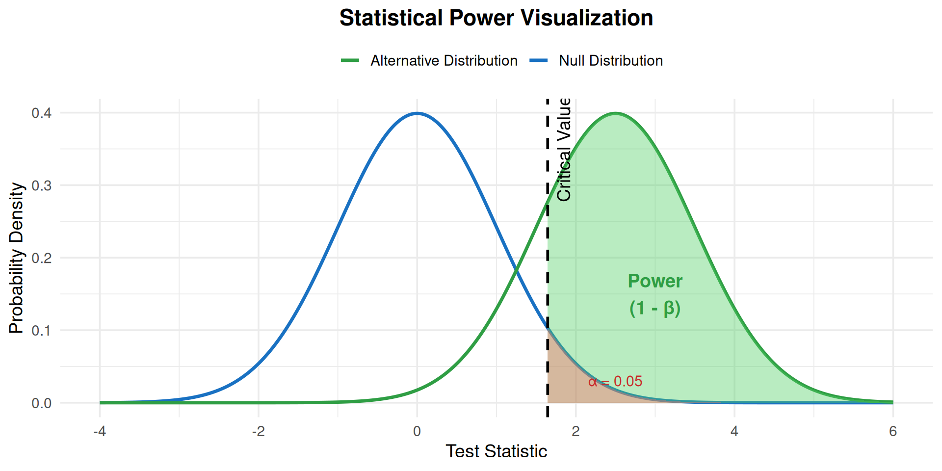
## Power in Context
```{r}
#| echo: false
#| fig-width: 10
#| fig-height: 5
#| fig-cap: "Visualization of statistical power showing the relationship between null and alternative distributions"
# Create visualization
x <- seq(-4, 6, length.out = 1000)
null_dist <- dnorm(x, mean = 0, sd = 1)
alt_dist <- dnorm(x, mean = 2.5, sd = 1)
# Critical value for alpha = 0.05
crit_val <- qnorm(0.95, mean = 0, sd = 1)
# Create data frame
df <- data.frame(
x = x,
null = null_dist,
alternative = alt_dist
)
ggplot(df, aes(x = x)) +
geom_line(aes(y = null, color = "Null Distribution"), linewidth = 1.2) +
geom_line(aes(y = alternative, color = "Alternative Distribution"), linewidth = 1.2) +
geom_area(data = subset(df, x >= crit_val),
aes(y = alternative), fill = "#51cf66", alpha = 0.4) +
geom_area(data = subset(df, x >= crit_val & x <= 4),
aes(y = null), fill = "#ff6b6b", alpha = 0.4) +
geom_vline(xintercept = crit_val, linetype = "dashed", linewidth = 1) +
annotate("text", x = crit_val + 0.2, y = 0.35, label = "Critical Value", angle = 90) +
annotate("text", x = 3, y = 0.15, label = "Power\n(1 - β)", color = "#2f9e44", size = 5, fontface = "bold") +
annotate("text", x = 2.5, y = 0.03, label = "α = 0.05", color = "#c92a2a", size = 4) +
scale_color_manual(values = c("Null Distribution" = "#1971c2",
"Alternative Distribution" = "#2f9e44")) +
labs(x = "Test Statistic", y = "Probability Density",
title = "Statistical Power Visualization",
color = "") +
theme_minimal(base_size = 14) +
theme(legend.position = "top",
plot.title = element_text(hjust = 0.5, face = "bold"))
```
# Why Do Power Analysis? {background-color="#0056A7"}
## Critical Reasons
1. **Resource Efficiency**
- Avoid wasting time, money, and effort on underpowered studies
- Don't collect more data than necessary
2. **Ethical Considerations**
- Minimize participant burden and exposure to risks
- Ensure research has realistic chance of success
3. **Scientific Integrity**
- Detect meaningful effects when they exist
- Avoid publishing false negatives
4. **Funding Requirements**
- Grant agencies require power analyses
- Demonstrates research feasibility
## Consequences of Low Power
::: {.columns}
::: {.column width="50%"}
### Too Small Sample
- Miss effective interventions (Type II error)
- Waste teacher and student time
- Publish false negatives ("it doesn't work")
- Discourage future research on promising approaches
- Contribute to replication crisis
:::
::: {.column width="50%"}
### Too Large Sample
- Unnecessary recruitment burden on schools
- Waste limited education funding
- Find statistically significant but educationally trivial results
- Fewer resources for other important studies
:::
:::
## Power Analysis is NOT About Gaming the System
::: {.callout-warning}
### Common Misconceptions
Power analysis should **help determine if a question can be reasonably answered**, not:
- Justify a predetermined sample size
- Defend what you want to study anyway
- Manipulate effect sizes to get funding
- Written defensively after the study is planned
:::
# The Logic of Power Analysis {background-color="#0056A7"}
## Five Key Components
Every power analysis involves specifying values for:
1. **Significance Level (α)**: Usually 0.05
2. **Power (1 - β)**: Usually 0.80 (minimum 80%)
3. **Effect Size (δ)**: Meaningful difference to detect
4. **Variability (σ)**: Standard deviation of measurements
5. **Sample Size (n)**: What we usually solve for
::: {.callout-note}
If you know any four, you can calculate the fifth!
:::
## Significance Level (α)
- **Type I error rate** - probability of false positive
- Conventionally set at **α = 0.05** (5%)
- Controls how "strict" we are about declaring effects significant
- Relates to **critical value** for hypothesis testing
```{r}
#| echo: true
# Critical value for one-tailed test, alpha = 0.05
qnorm(0.95)  # z = 1.645
# Critical value for two-tailed test, alpha = 0.05
qnorm(0.975)  # z = 1.96
```
## Power (1 - β)
- **Probability of detecting a true effect**
- Conventionally set at **0.80** (80%) or higher
- Higher power = more certainty in detecting effects
- Common choices: 70%, 80%, 90%
::: {.callout-important}
### Minimum Standards
- **80% power** is considered minimum acceptable
- **90% power** for clinical trials or high-stakes research
- Choice depends on how certain you want to be
:::
## Effect Size (δ)
The **meaningful difference** you want to detect
Must be specified based on:
- Prior research literature
- **Educational/practical significance** (not just statistical)
- Subject matter expertise
- Pilot data
::: {.callout-tip}
### Cohen's d (Standardized Effect Size)
Often expressed as: $d = \frac{|\delta|}{\sigma}$ (effect size relative to SD)
- **Small effect:** d ≈ 0.2 (subtle but meaningful in education)
- **Medium effect:** d ≈ 0.5 (typical for many interventions)
- **Large effect:** d ≈ 0.8 (rare in education research)
**Reality check:** Most education interventions have d = 0.2-0.4
:::
## Variability (σ)
**Standard deviation** of measurements
Estimate from:
- Prior published research
- Pilot studies
- Similar studies in literature
- Expert knowledge
::: {.callout-warning}
### Impact on Sample Size
Sample size increases proportionally to variance:
$$n \propto \sigma^2$$
**Doubling the SD quadruples the required sample size!**
:::
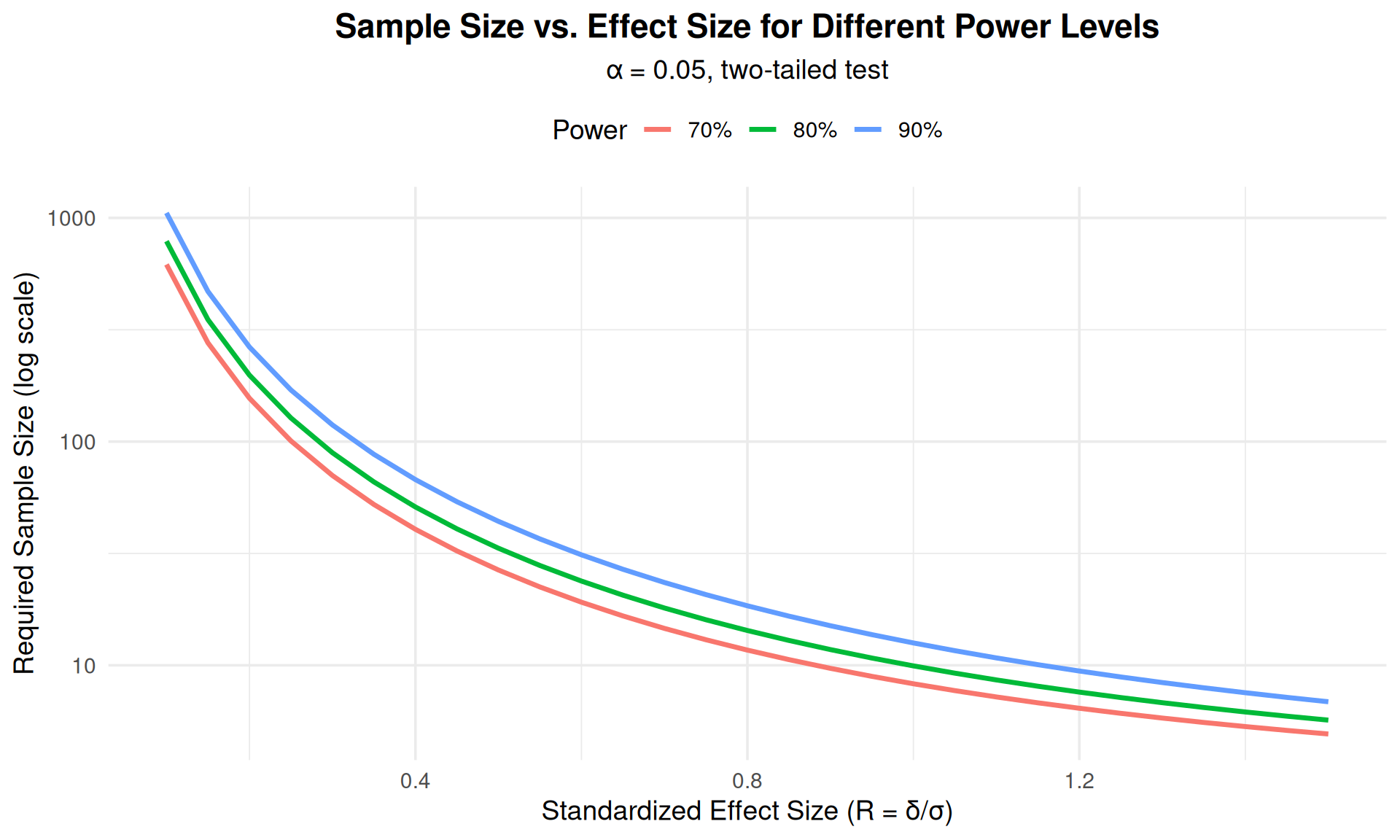
## Relationships Among Components
```{r}
#| echo: false
#| fig-width: 10
#| fig-height: 6
# Create data for different scenarios
effect_sizes <- seq(0.1, 1.5, by = 0.05)
power_70 <- sapply(effect_sizes, function(d) {
pwr.t.test(d = d, sig.level = 0.05, power = 0.70,
type = "one.sample", alternative = "two.sided")$n
})
power_80 <- sapply(effect_sizes, function(d) {
pwr.t.test(d = d, sig.level = 0.05, power = 0.80,
type = "one.sample", alternative = "two.sided")$n
})
power_90 <- sapply(effect_sizes, function(d) {
pwr.t.test(d = d, sig.level = 0.05, power = 0.90,
type = "one.sample", alternative = "two.sided")$n
})
df_power <- data.frame(
effect_size = rep(effect_sizes, 3),
sample_size = c(power_70, power_80, power_90),
power = rep(c("70%", "80%", "90%"), each = length(effect_sizes))
)
ggplot(df_power, aes(x = effect_size, y = sample_size, color = power)) +
geom_line(linewidth = 1.2) +
scale_y_log10() +
labs(x = "Standardized Effect Size (R = δ/σ)",
y = "Required Sample Size (log scale)",
title = "Sample Size vs. Effect Size for Different Power Levels",
subtitle = "α = 0.05, two-tailed test",
color = "Power") +
theme_minimal(base_size = 14) +
theme(legend.position = "top",
plot.title = element_text(hjust = 0.5, face = "bold"),
plot.subtitle = element_text(hjust = 0.5))
```
## Understanding (σ/δ)²: The Signal-to-Noise Ratio
::: {.callout-note icon=false}
### Why Does Sample Size Depend on (σ/δ)²?
The ratio **σ/δ** represents **noise-to-signal**:
- **δ** = effect size (the "signal" you want to detect)
- **σ** = variability (the "noise" that obscures the signal)
**Intuitive examples:**
| Scenario | δ | σ | σ/δ | Interpretation | n needed |
|----------|---|---|-----|----------------|----------|
| Strong signal, low noise | 10 | 5 | 0.5 | Easy to detect | Small |
| Weak signal, low noise | 5 | 5 | 1.0 | Moderate | Medium |
| Weak signal, high noise | 5 | 20 | 4.0 | Hard to detect | Large |
**Why squared?**
- Doubling noise (σ) means 4× more participants needed
- Halving effect size (δ) means 4× more participants needed
- This quadratic relationship comes from variance, not an arbitrary choice!
:::
## Key Facts to Remember
::: {.incremental}
1. **Sample size increases with power**: More power → larger sample needed
2. **Sample size increases with smaller detectable differences**: Smaller effect → larger sample (quadratically!)
3. **Sample size increases with variance**: More variability → larger sample (quadratically!)
4. **One-sided tests require smaller samples** than two-sided tests
5. **The (z_α + z_β)² term** represents the required distance between distributions
6. **The (σ/δ)² term** represents the signal-to-noise ratio
:::
# Power Analysis: One-Sample Case {background-color="#0056A7"}
## One-Sample Situation
Testing if a mean differs from a known value:
- $H_0: \mu = \mu_0$ (null hypothesis)
- $H_1: \mu \neq \mu_0$ or $\mu < \mu_0$ or $\mu > \mu_0$ (alternative)
**Required sample size formula:**
$$n = (z_\alpha + z_\beta)^2 \left(\frac{\sigma}{\delta}\right)^2$$
where:
- $z_\alpha$ = critical value for significance level
- $z_\beta$ = critical value for power
- $\delta = \mu_1 - \mu_0$ = effect size
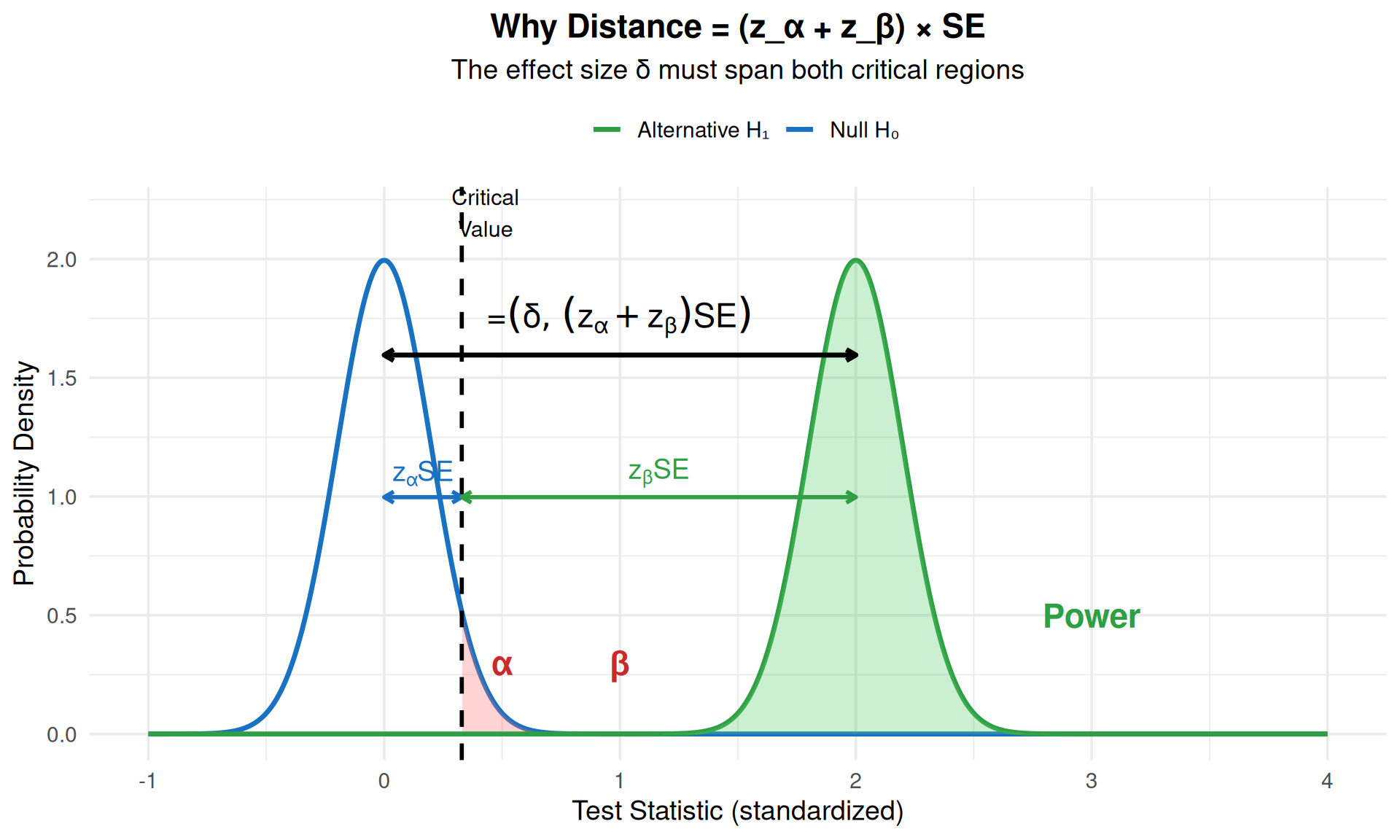
## Where Does This Formula Come From?
::: {.callout-note icon=false}
### The Logic Behind the Formula
**Key insight:** The distributions under H₀ and H₁ must be separated enough that:
1. The critical value from H₀ cuts off α (Type I error)
2. The critical value from H₁ cuts off β (Type II error)
**The distance between distributions** (in standard error units) must span both critical values:
$$\frac{\delta}{SE} = z_\alpha + z_\beta$$
Since $SE = \frac{\sigma}{\sqrt{n}}$, we have:
$$\frac{\delta}{\sigma/\sqrt{n}} = z_\alpha + z_\beta$$
Solving for n:
$$\sqrt{n} = \frac{(z_\alpha + z_\beta) \cdot \sigma}{\delta}$$
Square both sides:
$$n = (z_\alpha + z_\beta)^2 \left(\frac{\sigma}{\delta}\right)^2$$
:::
## Visual Intuition
```{r}
#| echo: false
#| fig-width: 10
#| fig-height: 6
# Create visualization showing why we need distance = z_alpha + z_beta
library(ggplot2)
# Parameters
mu0 <- 0
delta <- 2
sigma <- 1
n <- 25 # sample size
se <- sigma / sqrt(n)
# Create distributions
x <- seq(-1, 4, length.out = 1000)
null_dist <- dnorm(x, mean = mu0, sd = se)
alt_dist <- dnorm(x, mean = mu0 + delta, sd = se)
# Critical value for alpha = 0.05 (one-tailed)
z_alpha <- qnorm(0.95)
crit_val <- mu0 + z_alpha * se
# Calculate where this cuts the alternative distribution
z_beta_actual <- (crit_val - (mu0 + delta)) / se
power_actual <- pnorm(z_beta_actual, lower.tail = TRUE)
# Create data frame
df <- data.frame(
x = x,
null = null_dist,
alternative = alt_dist
)
# Create plot
ggplot(df, aes(x = x)) +
# Null distribution
geom_line(aes(y = null, color = "Null H₀"), linewidth = 1.2) +
geom_area(data = subset(df, x >= crit_val & x <= 1),
aes(y = null), fill = "#ff6b6b", alpha = 0.3) +
# Alternative distribution
geom_line(aes(y = alternative, color = "Alternative H₁"), linewidth = 1.2) +
geom_area(data = subset(df, x >= crit_val),
aes(y = alternative), fill = "#51cf66", alpha = 0.3) +
geom_area(data = subset(df, x < crit_val),
aes(y = alternative), fill = "#ff6b6b", alpha = 0.3) +
# Critical value line
geom_vline(xintercept = crit_val, linetype = "dashed", linewidth = 1) +
# Annotations showing distances
annotate("segment", x = mu0, xend = crit_val,
y = max(null_dist) * 0.5, yend = max(null_dist) * 0.5,
arrow = arrow(ends = "both", length = unit(0.2, "cm")),
color = "#1971c2", linewidth = 1) +
annotate("text", x = (mu0 + crit_val)/2, y = max(null_dist) * 0.55,
label = "z[α] * SE", parse = TRUE, color = "#1971c2", size = 5, fontface = "bold") +
annotate("segment", x = crit_val, xend = mu0 + delta,
y = max(alt_dist) * 0.5, yend = max(alt_dist) * 0.5,
arrow = arrow(ends = "both", length = unit(0.2, "cm")),
color = "#2f9e44", linewidth = 1) +
annotate("text", x = (crit_val + mu0 + delta)/2, y = max(alt_dist) * 0.55,
label = "z[β] * SE", parse = TRUE, color = "#2f9e44", size = 5, fontface = "bold") +
# Total distance
annotate("segment", x = mu0, xend = mu0 + delta,
y = max(alt_dist) * 0.8, yend = max(alt_dist) * 0.8,
arrow = arrow(ends = "both", length = unit(0.2, "cm")),
color = "black", linewidth = 1.2) +
annotate("text", x = mu0 + delta/2, y = max(alt_dist) * 0.88,
label = "δ = (z[α] + z[β]) * SE", parse = TRUE,
size = 6, fontface = "bold") +
# Labels
annotate("text", x = crit_val + 0.1, y = max(null_dist) * 1.1,
label = "Critical\nValue", angle = 0, size = 4) +
annotate("text", x = 0.5, y = max(null_dist) * 0.15,
label = "α", color = "#c92a2a", size = 6, fontface = "bold") +
annotate("text", x = 1, y = max(alt_dist) * 0.15,
label = "β", color = "#c92a2a", size = 6, fontface = "bold") +
annotate("text", x = 3, y = max(alt_dist) * 0.25,
label = "Power", color = "#2f9e44", size = 6, fontface = "bold") +
scale_color_manual(values = c("Null H₀" = "#1971c2", "Alternative H₁" = "#2f9e44")) +
labs(x = "Test Statistic (standardized)",
y = "Probability Density",
title = "Why Distance = (z_α + z_β) × SE",
subtitle = "The effect size δ must span both critical regions",
color = "") +
theme_minimal(base_size = 14) +
theme(legend.position = "top",
plot.title = element_text(hjust = 0.5, face = "bold"),
plot.subtitle = element_text(hjust = 0.5))
```
::: {.callout-tip}
### The Key Insight
The formula squared because:
1. We need: $\delta = (z_\alpha + z_\beta) \times SE$
2. Since $SE = \sigma/\sqrt{n}$, we have: $\delta = (z_\alpha + z_\beta) \times \frac{\sigma}{\sqrt{n}}$
3. Rearranging for $\sqrt{n}$: $\sqrt{n} = \frac{(z_\alpha + z_\beta) \times \sigma}{\delta}$
4. **Squaring both sides** to isolate n: $n = \frac{(z_\alpha + z_\beta)^2 \times \sigma^2}{\delta^2}$
The squaring comes from solving for n, not from squaring the sum first!
:::
## Example: Reading Achievement Study
::: {.callout-note icon=false}
### Research Question
Do students in a new literacy program have higher reading scores compared to the national average?
**Known Information:**
- National average reading score: μ₀ = 100
- Standard deviation: σ = 20
- Meaningful difference: δ = 5 points (improvement)
- Desired power: 80%
- Significance level: α = 0.05 (one-tailed)
:::
## Calculating Sample Size: Step by Step
```{r}
#| echo: true
#| results: hold
# Given values
mu0 <- 100      # national average score
sigma <- 20     # standard deviation
delta <- 5      # meaningful improvement
alpha <- 0.05   # significance level
power <- 0.80   # desired power

# Step 1: Find critical values
z_alpha <- qnorm(1 - alpha)  # = 1.645 for one-tailed
z_beta <- qnorm(power)       # = 0.842 for 80% power

cat("Step 1: Critical values\n")
cat("  z_alpha =", round(z_alpha, 3), "\n")
cat("  z_beta  =", round(z_beta, 3), "\n\n")

# Step 2: Calculate required distance (in SE units)
required_distance <- z_alpha + z_beta
cat("Step 2: Required distance between distributions\n")
cat("  z_alpha + z_beta =", round(required_distance, 3), "standard errors\n\n")

# Step 3: Set up the equation
# We need: delta = required_distance × SE
# We need: delta = required_distance × (sigma / sqrt(n))
# Solve for sqrt(n)
sqrt_n <- required_distance * sigma / delta
cat("Step 3: Solve for sqrt(n)\n")
cat("  sqrt(n) = (", round(required_distance, 3), " × ", sigma, ") / ", delta, "\n")
cat("  sqrt(n) =", round(sqrt_n, 3), "\n\n")

# Step 4: Square to get n
n <- sqrt_n^2
cat("Step 4: Square to get n\n")
cat("  n = (", round(sqrt_n, 3), ")²\n")
cat("  n =", round(n, 2), "\n\n")

cat("Required sample size:", ceiling(n), "students")
```
## Formula Summary: What Each Part Means
$$n = \underbrace{(z_\alpha + z_\beta)^2}_{\text{Separation needed}} \times \underbrace{\left(\frac{\sigma}{\delta}\right)^2}_{\text{Signal-to-noise}}$$
::: {.columns}
::: {.column width="50%"}
### $(z_\alpha + z_\beta)^2$
**What it controls:**
- Type I error (α)
- Type II error (β)
- Power (1 - β)
**Typical values:**
- α = 0.05, Power = 80%
- z_α = 1.645, z_β = 0.842
- Sum = 2.487
- $(z_\alpha + z_\beta)^2 \approx 6.2$
:::
::: {.column width="50%"}
### $(\sigma/\delta)^2$
**What it controls:**
- Effect size you want to detect (δ)
- Population variability (σ)
**Typical values:**
- Small effect: σ/δ = 5 → 25
- Medium effect: σ/δ = 2 → 4
- Large effect: σ/δ = 1.25 → 1.6
**Total:** n = 6.2 × (σ/δ)²
:::
:::
## Using the `pwr` Package
```{r}
#| echo: true
# Effect size (standardized)
effect_size <- abs(delta) / sigma

# Power analysis using pwr package
result <- pwr.t.test(
  d = effect_size,
  sig.level = alpha,
  power = power,
  type = "one.sample",
  alternative = "greater"  # or "two.sided", "less", "greater"
)

print(result)
# Verify our manual calculation matches
cat("\nManual calculation:",
    ceiling(n),
    "\npwr package:",
    abs(ceiling(result$n)))
```
## Paired Comparisons
The one-sample formula applies to **paired (blocked) designs**:
Response: $D = Y_2 - Y_1$ (difference between paired measurements)
Examples:
- Pre-test vs. Post-test
- Treatment vs. Control on same subject
- Left eye vs. Right eye
**Key:** Need SD of the **differences**, not individual measurements
## Example: Pre-Post Test Anxiety Study
::: {.callout-note icon=false}
### Research Question
Does a mindfulness intervention reduce student test anxiety?
**Study Design:**
- Paired comparison: post-intervention vs. baseline on same students
- SD of differences: σ = 5 points
- Meaningful reduction: δ = -2.5 points
- Power: 80%, α = 0.05
:::
```{r}
#| echo: true
# Calculate sample size for paired comparison
sigma_diff <- 5.0
delta_anxiety <- -2.5
effect <- abs(delta_anxiety) / sigma_diff

pwr.t.test(d = effect, sig.level = 0.05, power = 0.80,
           type = "paired", alternative = "two.sided")
```
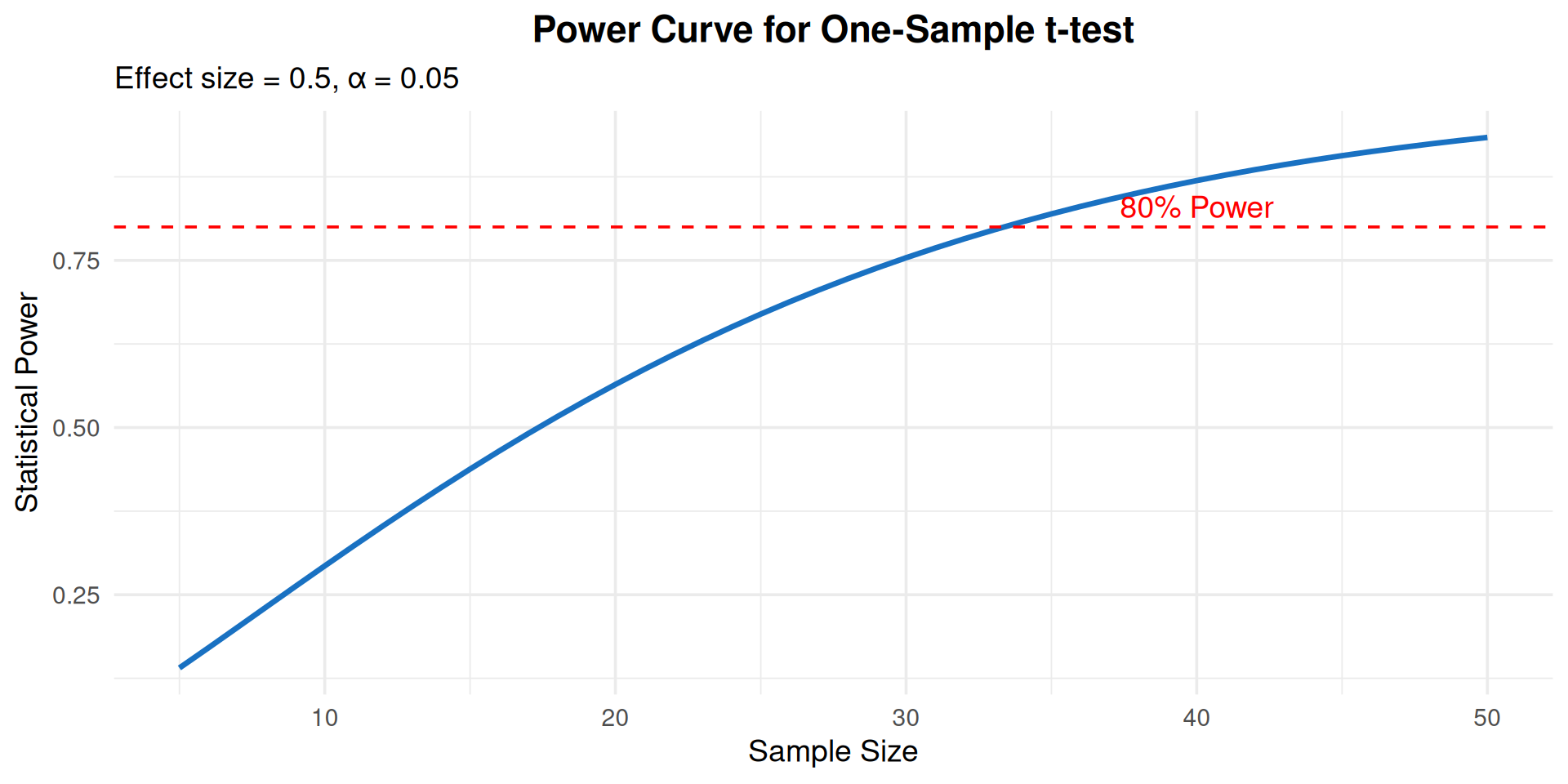
## Exploring Power Curves
```{r}
#| echo: true
#| fig-width: 10
#| fig-height: 5
# Create power curve for different sample sizes
sample_sizes <- seq(5, 50, by = 1)
effect_size <- 0.5

power_values <- sapply(sample_sizes, function(n) {
  pwr.t.test(n = n, d = effect_size, sig.level = 0.05,
             type = "one.sample", alternative = "two.sided")$power
})

ggplot(data.frame(n = sample_sizes, power = power_values),
       aes(x = n, y = power)) +
  geom_line(linewidth = 1.2, color = "#1971c2") +
  geom_hline(yintercept = 0.80, linetype = "dashed", color = "red") +
  annotate("text", x = 40, y = 0.83, label = "80% Power", color = "red") +
  labs(x = "Sample Size", y = "Statistical Power",
       title = "Power Curve for One-Sample t-test",
       subtitle = "Effect size = 0.5, α = 0.05") +
  theme_minimal(base_size = 14) +
  theme(plot.title = element_text(hjust = 0.5, face = "bold"))
```
# Power Analysis: Two-Sample Case {background-color="#0056A7"}
## Two-Sample Comparison
Comparing means of two independent groups:
- $H_0: \mu_2 - \mu_1 = 0$
- $H_1: \mu_2 - \mu_1 \neq 0$ (or $<$ or $>$)
**Both means are unknown** - different from one-sample case!
## Two-Sample Formulas
### Case 1: Unequal Variances
**Total sample size:**
$$N = (z_\alpha + z_\beta)^2 \left[\frac{\sigma_1 + \sigma_2}{\delta}\right]^2$$
Allocate samples proportional to SDs:
$$n_1 = N \cdot \frac{\sigma_1}{\sigma_1 + \sigma_2}, \quad n_2 = N \cdot \frac{\sigma_2}{\sigma_1 + \sigma_2}$$
### Case 2: Equal Variances
**Sample size per group:**
$$n = 2(z_\alpha + z_\beta)^2 \left(\frac{\sigma}{\delta}\right)^2$$
## Example: Math Achievement by SES
::: {.callout-note icon=false}
### Research Question
Compare math achievement scores between students from high and low socioeconomic status (SES) backgrounds
**Known Information:**
- High SES group: σ₁ = 12 points
- Low SES group: σ₂ = 15 points (larger variability)
- Meaningful difference: δ = 10 points
- Power: 80%, α = 0.05
:::
## Calculation: Unequal Variances
```{r}
#| echo: true
# Given values
sigma1 <- 12    # High SES SD
sigma2 <- 15    # Low SES SD
delta <- 10     # Effect size
alpha <- 0.05
power <- 0.80

# Critical values
z_alpha <- qnorm(1 - alpha/2, lower.tail = TRUE)  # two-tailed
z_beta <- qnorm(power, lower.tail = TRUE)

# Total sample size
N <- (z_alpha + z_beta)^2 * ((sigma1 + sigma2) / delta)^2

# Allocate proportional to SDs
n1 <- ceiling(N * sigma1 / (sigma1 + sigma2))
n2 <- ceiling(N * sigma2 / (sigma1 + sigma2))

cat("High SES students:", n1, "\n")
cat("Low SES students:", n2, "\n")
cat("Total sample size:", n1 + n2)
```
## Using `pwr` for Two-Sample Tests
```{r}
#| echo: true
# For equal variances (using larger SD as planning value)
sigma <- sqrt((sigma1^2 + sigma2^2)/2) # pooled standard deviation
effect_size <- abs(delta) / sigma # Cohen' d

result <- pwr.t.test(
  d = effect_size,
  sig.level = 0.05,
  power = 0.80,
  type = "two.sample",
  alternative = "two.sided"
)

print(result)
cat("\nTotal sample size:", ceiling(result$n * 2))
```
## Example: Study Skills Workshop
::: {.callout-note icon=false}
### Research Question
Does a study skills workshop improve GPA compared to no intervention?
**Study Design:**
- Two independent groups (workshop vs. control)
- Equal SDs: σ = 0.5 GPA points
- Meaningful change: δ = 0.3 GPA points
- Power: 80%, α = 0.05
:::
```{r}
#| echo: true
sigma <- 0.5
delta <- 0.3
effect_size <- delta / sigma

pwr.t.test(d = effect_size, sig.level = 0.05, power = 0.80,
           type = "two.sample", alternative = "two.sided")
```
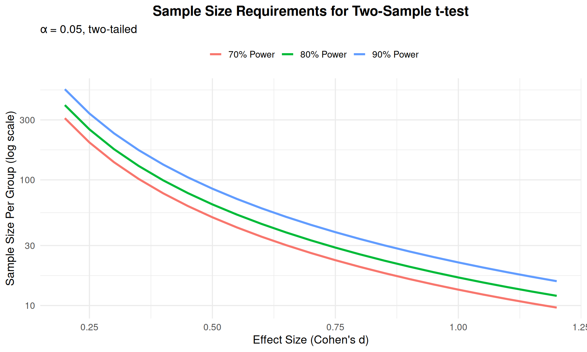
## Visualizing Two-Sample Power
```{r}
#| echo: false
#| fig-width: 10
#| fig-height: 6
# Create comprehensive power analysis plot
effect_sizes <- seq(0.2, 1.2, by = 0.05)
powers <- c(0.70, 0.80, 0.90)
results <- expand.grid(effect = effect_sizes, power = powers)
results$n_per_group <- sapply(1:nrow(results), function(i) {
pwr.t.test(d = results$effect[i],
power = results$power[i],
sig.level = 0.05,
type = "two.sample")$n
})
results$power_label <- paste0(results$power * 100, "% Power")
ggplot(results, aes(x = effect, y = n_per_group, color = power_label)) +
geom_line(linewidth = 1.2) +
scale_y_log10() +
labs(x = "Effect Size (Cohen's d)",
y = "Sample Size Per Group (log scale)",
title = "Sample Size Requirements for Two-Sample t-test",
subtitle = "α = 0.05, two-tailed",
color = "") +
theme_minimal(base_size = 14) +
theme(legend.position = "top",
plot.title = element_text(hjust = 0.5, face = "bold"))
```
# Power Analysis: Other Designs {background-color="#0056A7"}
## Log-Normal Distributions
When data are **log-normally distributed**:
- Easier to specify effects as **percentage changes**
- Variability expressed as **coefficient of variation**
$$c = \frac{\sqrt{\text{Var}(Y)}}{E(Y)}$$
**Sample size per group:**
$$n = \frac{2(z_\alpha + z_\beta)^2 c^2}{[\log(1+f)]^2}$$
where $f$ is the proportionate change (e.g., 0.20 for 20% increase)
## Example: Reaction Time Study
::: {.callout-note icon=false}
### Research Question
Compare reaction times between students with ADHD receiving medication vs. placebo
**Known Information:**
- Coefficient of variation: c = 0.30
- Expected difference: 20% faster reaction time with medication (f = -0.20)
- Power: 80%, α = 0.05
*Note: Reaction times typically follow log-normal distributions*
:::
```{r}
#| echo: true
# Given values
c <- 0.30       # Coefficient of variation
f <- 0.20       # 20% proportionate change
alpha <- 0.05
power <- 0.80

# Critical values
z_alpha <- qnorm(alpha, lower.tail = TRUE)
z_beta <- qnorm(1 - power, lower.tail = TRUE)

# Sample size calculation
n <- 2 * (z_alpha + z_beta)^2 * c^2 / (log(1 + f))^2
cat("Sample size per group:", ceiling(n), "\n")
cat("Total sample size:", ceiling(n) * 2)
```
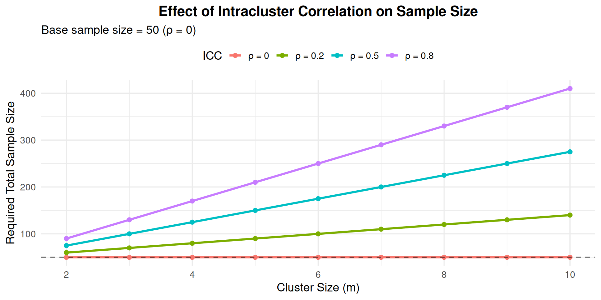
## Cluster Randomized Designs
**Clusters** = groups of experimental units
Common examples:
- In education: Students within classrooms, classrooms within schools
- Also: Patients within clinics, siblings within families
**Intracluster Correlation (ρ):**
- Measures similarity within clusters
- Range: 0 to 1
- ρ = 0: units independent (no clustering effect)
- ρ = 1: units identical within cluster
- **Typical values in education:** 0.10-0.25 for students in classrooms
**Sample size adjustment:**
$$n = km = 2(z_\alpha + z_\beta)^2 \left(\frac{\sigma}{\delta}\right)^2 [1 + (m-1)\rho]$$
where $k$ = number of clusters, $m$ = units per cluster
## Impact of Intracluster Correlation
```{r}
#| echo: false
#| fig-width: 10
#| fig-height: 5
# Show how ICC affects sample size
cluster_sizes <- 2:10
icc_values <- c(0, 0.2, 0.5, 0.8)
# Base sample size (no clustering)
base_n <- 50
results <- expand.grid(m = cluster_sizes, rho = icc_values)
results$n_required <- base_n * (1 + (results$m - 1) * results$rho)
results$rho_label <- paste0("ρ = ", results$rho)
ggplot(results, aes(x = m, y = n_required, color = rho_label)) +
geom_line(linewidth = 1.2) +
geom_point(size = 2) +
geom_hline(yintercept = base_n, linetype = "dashed", alpha = 0.5) +
labs(x = "Cluster Size (m)",
y = "Required Total Sample Size",
title = "Effect of Intracluster Correlation on Sample Size",
subtitle = "Base sample size = 50 (ρ = 0)",
color = "ICC") +
theme_minimal(base_size = 14) +
theme(legend.position = "top",
plot.title = element_text(hjust = 0.5, face = "bold"))
```
## Cluster Design: Key Insights
::: {.incremental}
1. **High ICC → Need more clusters, not more units per cluster**
- With ρ = 0.20, adding more students per classroom doesn't help proportionally
- Better to recruit more classrooms with fewer students each
- In education research, typical ICC for classrooms: 0.10-0.25
2. **Ignoring ICC leads to underpowered studies**
- Don't calculate as if students are independent
- Must account for clustering in design
- Failure to account for ICC is a common error in educational research
3. **Design Efficiency**
- Maximize number of clusters (k = classrooms, schools)
- Consider cluster size (m) and practical constraints
- Balance statistical needs with recruitment feasibility
:::
## Example: Students in Classrooms
::: {.callout-note icon=false}
### Scenario
- Need 100 students total with ρ = 0.20
- Cluster size m = 20 (students per classroom)
**Incorrect approach (ignoring ICC):**
$$n = 100 \text{ students} \rightarrow 5 \text{ classrooms}$$
**Correct approach (accounting for ICC):**
$$n = 100 \times [1 + (20-1)(0.20)] = 100 \times 4.8 = 480 \text{ students}$$
$$\rightarrow 24 \text{ classrooms needed (12 per condition)}$$
:::
::: {.callout-warning}
Always account for clustering structure in your design!
:::
# Power Analysis: ANOVA Designs {background-color="#0056A7"}
## One-Way ANOVA
Comparing means across **multiple groups** (k ≥ 3)
**Effect size (f):**
$$f = \frac{\sigma_{\text{between}}}{\sigma_{\text{within}}}$$
Conventional values:
- Small: f = 0.10
- Medium: f = 0.25
- Large: f = 0.40
## ANOVA Power Analysis in R
```{r}
#| echo: true
# Example: Comparing 4 groups
k <- 4              # number of groups
effect_size <- 0.25 # medium effect
alpha <- 0.05
power <- 0.80

# Power analysis
pwr.anova.test(
  k = k,
  f = effect_size,
  sig.level = alpha,
  power = power
)
```
## Factorial ANOVA
For **2×2 factorial design**:
- Two factors, each with 2 levels
- Tests main effects and interaction
::: {.callout-note}
**Note:** `pwr.f2.test()` returns `v` (denominator degrees of freedom). To get total sample size: $n = v + u + 1$
:::
```{r}
#| echo: true
# Effect size for factorial design
effect_size <- 0.25
alpha <- 0.05
power <- 0.80

# Numerator df = (levels - 1)
# For 2x2: df = 1 for each main effect and interaction

result <- pwr.f2.test(
  u = 1,              # numerator df for one effect
  f2 = effect_size^2, # f-squared effect size
  sig.level = alpha,
  power = power
)

print(result)
# Calculate total sample size from v (denominator df)
# Formula: n = v + u + 1
n_total <- ceiling(result$v + result$u + 1)
cat("\nTotal sample size needed:", n_total, "participants")
```
## Understanding pwr.f2.test Output
::: {.callout-tip}
### Interpreting the Results
When using `pwr.f2.test()`, the output shows:
- **u** = numerator degrees of freedom (number of predictors/effects tested)
- **v** = denominator degrees of freedom (error df)
- **f2** = Cohen's f² effect size
- **sig.level** = α level
- **power** = statistical power
**Important:** To get the total sample size needed:
$$n = v + u + 1$$
**Example:** If u = 1 and v = 125.53, you need n = 128 participants total.
:::
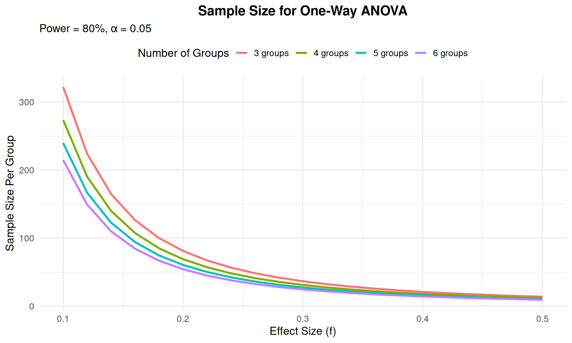
## Visualizing ANOVA Power
```{r}
#| echo: false
#| fig-width: 10
#| fig-height: 6
# Power curves for different numbers of groups
k_values <- c(3, 4, 5, 6)
effect_sizes <- seq(0.1, 0.5, by = 0.02)
results <- expand.grid(k = k_values, effect = effect_sizes)
results$n <- sapply(1:nrow(results), function(i) {
pwr.anova.test(k = results$k[i],
f = results$effect[i],
sig.level = 0.05,
power = 0.80)$n
})
results$k_label <- paste0(results$k, " groups")
ggplot(results, aes(x = effect, y = n, color = k_label)) +
geom_line(linewidth = 1.2) +
labs(x = "Effect Size (f)",
y = "Sample Size Per Group",
title = "Sample Size for One-Way ANOVA",
subtitle = "Power = 80%, α = 0.05",
color = "Number of Groups") +
theme_minimal(base_size = 14) +
theme(legend.position = "top",
plot.title = element_text(hjust = 0.5, face = "bold"))
```
# Power Analysis: Proportions and Correlations {background-color="#0056A7"}
## Comparing Two Proportions
Testing difference between two proportions (e.g., success rates)
**Effect size (h):**
$$h = 2[\arcsin(\sqrt{p_1}) - \arcsin(\sqrt{p_2})]$$
```{r}
#| echo: true
# Example: Compare graduation rates
p1 <- 0.70  # Control group
p2 <- 0.80  # Treatment group

# Calculate effect size
ES.h(p1, p2)
# Power analysis
pwr.2p.test(
  h = ES.h(p1, p2),
  sig.level = 0.05,
  power = 0.80,
  alternative = "two.sided"
)
```
## Testing Correlations
Testing if correlation differs from zero
**Effect size = r** (the correlation itself)
```{r}
#| echo: true
# Test if correlation r = 0.30 is significant
r <- 0.30

pwr.r.test(
  r = r,
  sig.level = 0.05,
  power = 0.80,
  alternative = "two.sided"
)
```
## Chi-Square Tests
For contingency tables:
**Effect size (w):**
- Small: w = 0.10
- Medium: w = 0.30
- Large: w = 0.50
```{r}
#| echo: true
# Example: 3x3 contingency table
df <- (3 - 1) * (3 - 1)  # degrees of freedom

pwr.chisq.test(
  w = 0.30,         # medium effect
  df = df,
  sig.level = 0.05,
  power = 0.80
)
```
# Software Tools for Power Analysis {background-color="#0056A7"}
## Available Software
::: {.columns}
::: {.column width="50%"}
### R Packages
- **`pwr`**: Most common for psychology/education
- **`WebPower`**: Web-based interface
- **`simr`**: Simulation-based for mixed models
- **`powerAnalysis`**: Educational resource
- **`clusterPower`**: Cluster randomized trials
:::
::: {.column width="50%"}
### Standalone Software
- **G*Power**: Free, widely used in psychology
- **Optimal Design**: Multilevel designs in education
- **PowerUpR**: R package for education research
- **PASS**: Commercial, extensive capabilities
- **Russell Lenth's applets**: Free online tools
:::
:::
## Using G*Power
Popular free software for power analysis:
1. Select test family (t-test, ANOVA, regression, etc.)
2. Choose specific test type
3. Specify:
- Effect size
- α level
- Power or sample size
4. Get results with visualizations
Download: [https://www.psychologie.hhu.de/arbeitsgruppen/allgemeine-psychologie-und-arbeitspsychologie/gpower](https://www.psychologie.hhu.de/arbeitsgruppen/allgemeine-psychologie-und-arbeitspsychologie/gpower)
# Practical Guidelines {background-color="#0056A7"}
## Before Running Your Study
::: {.incremental}
1. **Review literature** for:
- Expected effect sizes
- Variability estimates
- Similar study designs
2. **Consider pilot studies** to:
- Estimate parameters
- Test procedures
- Refine hypotheses
3. **Specify meaningful effects**:
- Clinical/practical significance
- Minimum detectable difference
- Cost-benefit considerations
:::
## Conducting Power Analysis
::: {.incremental}
1. **Be conservative**:
- Use realistic (not optimistic) effect sizes
- Account for attrition/dropout
- Consider multiple comparisons
2. **Perform sensitivity analysis**:
- Vary effect sizes
- Check impact of assumptions
- Explore "what if" scenarios
3. **Document everything**:
- Assumptions and their sources
- Calculations and software used
- Rationale for parameter choices
:::
## Common Pitfalls to Avoid
::: {.callout-warning}
### Don't:
1. Manipulate effect sizes to justify small samples
2. Ignore clustering or dependence
3. Use published effect sizes uncritically (publication bias!)
4. Forget about attrition/missing data
5. Conduct power analysis after data collection ("post-hoc power")
6. Ignore practical constraints (budget, time, recruitment)
:::
## Post-Hoc Power Analysis
::: {.callout-important}
### Why Not to Do It
**Post-hoc power analysis** (after collecting data) is controversial:
- Circular reasoning: uses observed effect to estimate power
- Non-significant results always have low post-hoc power
- Doesn't change interpretation of results
- Confidence intervals more informative
**Exception:** Informing future studies with pilot data
:::
# Applied Examples {background-color="#0056A7"}
## Example 1: Reading Intervention
::: {.callout-note icon=false}
### Research Question
Does a new reading intervention improve test scores compared to standard curriculum?
**Information:**
- Two independent groups (intervention vs. control)
- σ = 15 points (from prior studies)
- Meaningful improvement: 5 points
- Power: 80%, α = 0.05 (two-tailed)
:::
```{r}
#| echo: true
effect_size <- 5 / 15  # 0.333
pwr.t.test(d = effect_size, sig.level = 0.05, power = 0.80,
           type = "two.sample", alternative = "two.sided")
```
**Need ~143 students per group, 286 total**
## Example 2: Class Size Study
::: {.callout-note icon=false}
### Research Question
Do smaller class sizes improve student achievement? Compare 3 class size conditions.
**Information:**
- Three groups: Small (15), Medium (25), Large (35)
- σ = 10 points
- Expected η² = 0.06 (medium effect)
- Convert to f: $f = \sqrt{\frac{\eta^2}{1-\eta^2}} = 0.25$
:::
```{r}
#| echo: true
eta_squared <- 0.06
f <- sqrt(eta_squared / (1 - eta_squared))

pwr.anova.test(k = 3, f = f, sig.level = 0.05, power = 0.80)
```
**Need ~52 students per class, 156 total**
## Example 3: Correlation Study
::: {.callout-note icon=false}
### Research Question
Is there a significant correlation between homework time and GPA?
**Expected correlation:** r = 0.30 (medium)
:::
```{r}
#| echo: true
pwr.r.test(r = 0.30, sig.level = 0.05, power = 0.80,
           alternative = "two.sided")
```
**Need ~85 students**
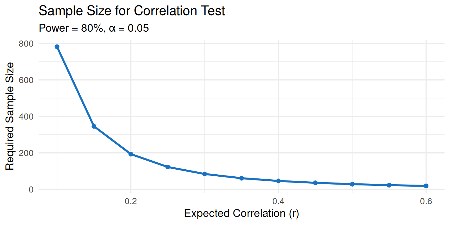
```{r}
#| echo: false
#| fig-width: 8
#| fig-height: 4
# Visualize power for different correlations
r_values <- seq(0.1, 0.6, by = 0.05)
n_values <- sapply(r_values, function(r) {
pwr.r.test(r = r, sig.level = 0.05, power = 0.80)$n
})
ggplot(data.frame(r = r_values, n = n_values),
aes(x = r, y = n)) +
geom_line(linewidth = 1.2, color = "#1971c2") +
geom_point(size = 2, color = "#1971c2") +
labs(x = "Expected Correlation (r)",
y = "Required Sample Size",
title = "Sample Size for Correlation Test",
subtitle = "Power = 80%, α = 0.05") +
theme_minimal(base_size = 14)
```
## Example 4: Multilevel Design
::: {.callout-note icon=false}
### Research Question
Testing intervention effects with students nested in classrooms
**Information:**
- 20 students per classroom
- ICC = 0.15 (typical for education)
- Effect size d = 0.40
:::
```{r}
#| echo: true
# Base sample size (ignoring clustering)
base <- pwr.t.test(d = 0.40, power = 0.80, sig.level = 0.05,
                   type = "two.sample")
base_n <- ceiling(base$n)

# Adjust for clustering
m <- 20           # cluster size
rho <- 0.15       # ICC
design_effect <- 1 + (m - 1) * rho

adjusted_n <- ceiling(base_n * design_effect)

cat("Base sample size per group:", base_n, "\n")
cat("Design effect:", round(design_effect, 2), "\n")
cat("Adjusted sample size per group:", adjusted_n, "\n")
cat("Number of classrooms needed per group:",
    ceiling(adjusted_n / m))
```
# Summary and Recommendations {background-color="#0056A7"}
## Key Takeaways
::: {.incremental}
1. **Power analysis is essential** for ethical, efficient research
2. **Minimum 80% power** to detect meaningful effects
3. **Four key inputs**: α, power, effect size, variability
4. **Sample size relationships**:
- Increases with desired power
- Increases quadratically with smaller effect sizes
- Increases with greater variability
5. **Account for study design**: clustering, pairing, multiple groups
:::
## Recommendations for Practice
::: {.columns}
::: {.column width="50%"}
### Planning Stage
- Conduct early in research design
- Use realistic effect sizes
- Consider attrition
- Perform sensitivity analyses
- Document all assumptions
:::
::: {.column width="50%"}
### Resources
- Use established software (pwr, G*Power)
- Consult statistician
- Review similar studies
- Conduct pilot studies
- Get peer review of power analysis
:::
:::
## Decision Framework
```{mermaid}
%%| fig-width: 10
flowchart TD
    A[Research Question] --> B{Feasible<br/>Sample Size?}
    B -->|Yes| C[Conduct Study]
    B -->|No| D{Can Increase<br/>Sample?}
    D -->|Yes| E[Revise Budget/<br/>Timeline]
    D -->|No| F{Can Accept<br/>Larger δ?}
    F -->|Yes| G[Revise Research<br/>Question]
    F -->|No| H[Abandon/<br/>Restructure]
    E --> C
    G --> C

    style C fill:#51cf66
    style H fill:#ff6b6b
```
## Further Reading
1. **Cohen, J. (1988).** *Statistical power analysis for the behavioral sciences* (2nd ed.). Routledge.
- The classic reference for power analysis in psychology and education
2. **Faul, F., Erdfelder, E., Lang, A. G., & Buchner, A. (2007).** G*Power 3: A flexible statistical power analysis program. *Behavior Research Methods, 39*, 175-191.
- Free software widely used in psychology and education
3. **Lakens, D. (2022).** Sample size justification. *Collabra: Psychology, 8*(1), 33267.
- Modern perspective on justifying sample sizes
4. **Spybrook, J., et al. (2011).** Optimal Design Plus Empirical Evidence: Documentation for the Optimal Design software.
- Specialized for cluster randomized trials in education
5. **Ledolter, J., & Kardon, R. (2020).** Focus on data: Statistical design of experiments and sample size selection using power analysis. *Investigative Ophthalmology & Visual Science, 61*(8), 11.
- General principles applicable across disciplines
# Questions? {background-color="#0056A7"}
## Resources and Practice
::: {.callout-tip}
### Practice Exercises
1. Calculate sample size for your own research question
2. Explore power curves with different parameters
3. Compare results across different software
4. Conduct sensitivity analysis
:::
### Contact Information
- Office Hours: [Schedule]
- Email: [Your email]
- Course Website: [Link]