“Click here to see R code”
dog_means <- c(19.25, 20.75, 22.25, 17.50, 18.75, 19.50 )
sum(4 * (dog_means - 19.67)^2)
[1] 54.3336Question: How about the research scenario when more than two independent variables?
Repeated measures ANOVA is one member of a much broader family of longitudinal designs — any study that collects data on the same units at multiple time points. These designs appear at two levels:
Data are collected from different (independent) samples at each wave, tracking population-level change over time rather than individuals.
Examples:
Key feature: Because different individuals are measured each wave, individual trajectories cannot be tracked — only group-level trends.
The same individuals are followed across time, enabling analysis of individual change trajectories and within-person variability.
Examples:
Key feature: Because the same person is measured repeatedly, observations are correlated — this is precisely the dependency that Repeated Measures ANOVA (and later, multilevel models) is designed to handle.
Note. All ANOVA-related designs talked about in this class can handle only one dependent variable; if you want to deal with more than 2 dependent variable, we may consider other research designs…
To conduct the hypothesis test, we follow:
Before conducting the hypothesis test, we check:
Independence of the observations:
| Tutoring Type | Time 1 (1st week out) | Time 2 (2nd week out) | Time 3 (3rd week out) |
|---|---|---|---|
| None | Sally Joe Montes |
Sally Joe Montes |
Sally Joe Montes |
| Once/week | Omar Fred Jenny |
Omar Fred Jenny |
Omar Fred Jenny |
| Daily | Chi Lena Caroline |
Chi Lena Caroline |
Chi Lena Caroline |
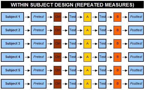
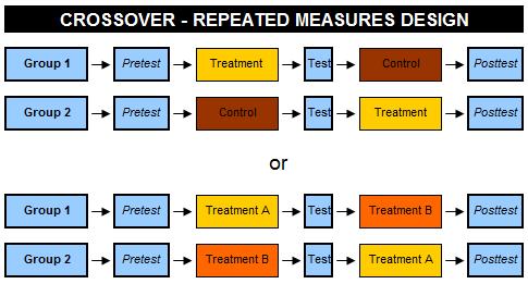
Two types of repeated measures are common:
Cross-over Design: alternatively, experiments can involve administering all treatment levels (in a sequence) to each experimental unit.
| Period 1 | Period 2 | |
|---|---|---|
| Sequence AB | A | B |
| Sequence BA | B | A |
How many potential sequences are for J x J design?
\prod (J, J-1, \cdots,1)
Two types of repeated measures are common:
| Period 1 | Period 2 | Period 3 | |
|---|---|---|---|
| Sequence ABC | A | B | C |
| Sequence BCA | B | C | A |
| Sequence CAB | C | A | B |
| Sequence ACB | A | C | B |
| Sequence BAC | B | A | C |
| Sequence CBA | C | B | A |
Carryover effects:
In a cross-over design, carryover effects refer to the residual effects of a treatment that persist and influence responses in subsequent treatment periods.
Since each participant receives multiple treatments in sequence, the outcome measured in a later period may be affected not only by the current treatment but also by the lingering influence of prior treatments.
✅ Example:
Discussion: Can you think about more carryover effect in your research area?
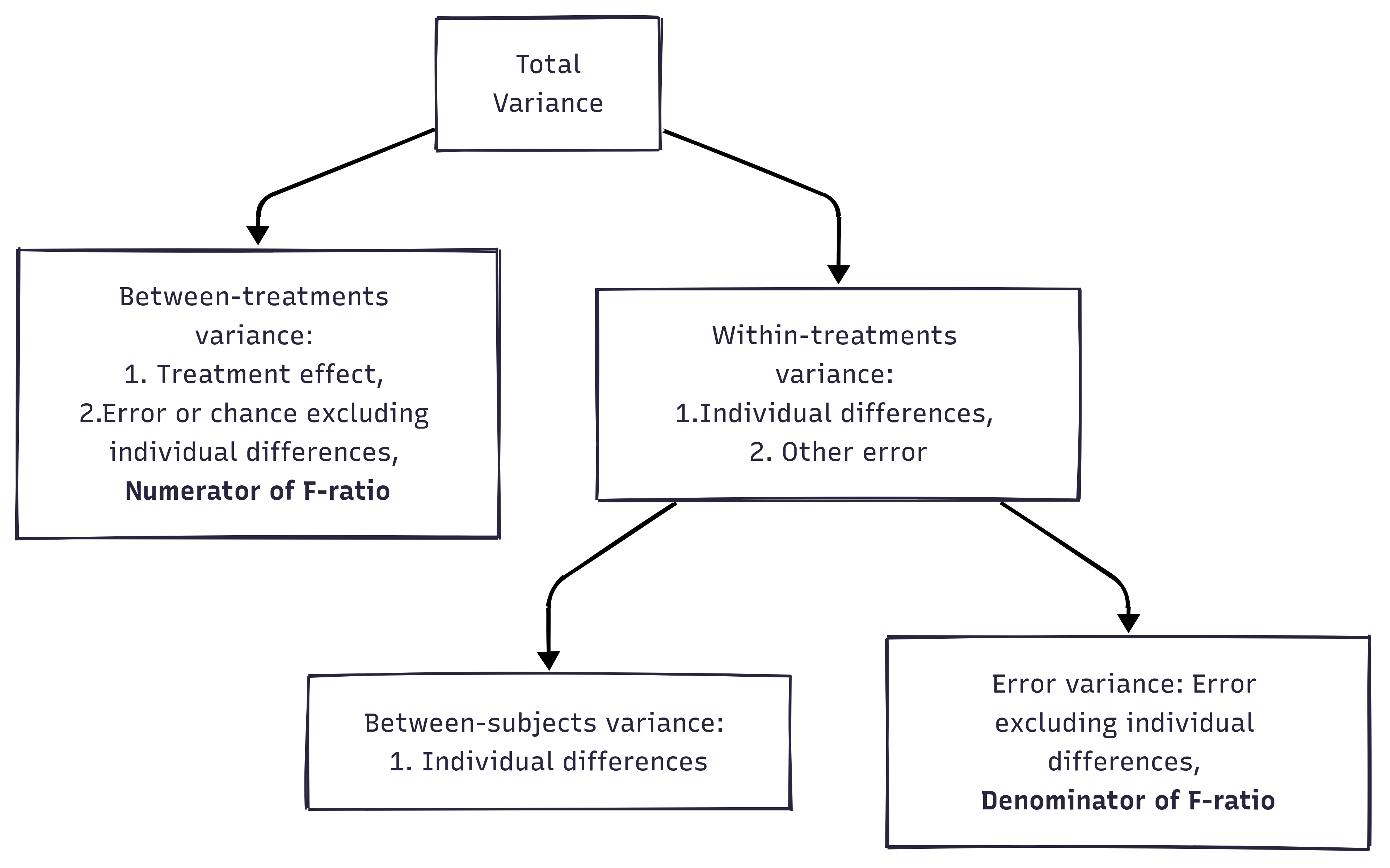
In RM ANOVA design, within-group variability (SSw) is used as the error variability (SSError).
The F-statistic is calculated as the ratio of MSModel to MSError:
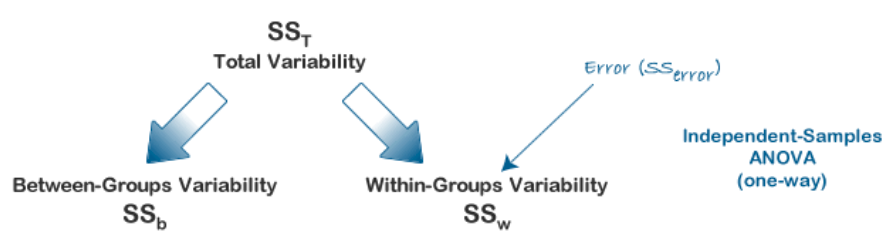
Independent ANOVA:
F = \frac{MS_b}{MS_w} = \frac{MS_b}{MS_{error}}
“Why subjects differ within the same group (e.g., treatment/control groups)” can be explained in RM ANOVA!
The advantage of a repeated measures ANOVA:
A repeated measures ANOVA calculates an F-statistic in a similar way:
 Generated by https://www.mermaidchart.com/app/projects
Mathematically, we are partitioning the variability attributable to the differences between groups (SSconditions) and variability within groups (SSw) exactly as we do in a between-subjects (independent) ANOVA.
With a repeated measures ANOVA, we are using the same subjects in each group, so we can remove the variability due to the individual differences between subjects, referred to as SSsubjects, from the within-groups variability (SSw).
We simply treat each subject as a “block.”
The ability to subtract SSsubjects will leave us with a smaller SSerror term:
Independent ANOVA: SS_{error} = SS_{w}
Repeated Measures ANOVA: SS_{error} = SS_{w} - SS_{subjects}
Background: Histamine is an organic nitrogenous compound produced by immune cells (mast cells and basophils) to fight invaders.
| Dog ID | time1 | time2 | time3 | time4 | Dog mean |
|---|---|---|---|---|---|
| 1 | 10 | 16 | 25 | 26 | 19.25 |
| 2 | 12 | 19 | 27 | 25 | 20.75 |
| 3 | 13 | 20 | 28 | 28 | 22.25 |
| 4 | 12 | 18 | 25 | 15 | 17.50 |
| 5 | 11 | 20 | 26 | 18 | 18.75 |
| 6 | 10 | 22 | 27 | 19 | 19.50 |
| Time mean | 11.33 | 19.17 | 26.33 | 21.83 | Grand mean = 19.67 |
| Component | Source | Sub-Component | SS | df | MS | F |
|---|---|---|---|---|---|---|
| I | Between-time | |||||
| II | Within-time | Between-Subjects | ||||
| III | Within-time | Within-Subjects / Error |
Note. Under the repeated measures ANOVA, we can decompose the total variability:
Total variability of DV = “between-time” variability + “within-time” variability
Between-subjects are useful because we can use it to explain the treatment effects / gender effects (anything relevant to why people different from each other).
Question this component answers: Do average histamine levels differ across the four time points?
For each time point, we measure how far its average is from the grand average of all measurements, then multiply by the number of dogs (6). Summing these squared distances gives SS_{btime} = 712.96.
We calculate mean square for between-time as:
MS_{btime} = \frac{SS_{btime}}{df_{btime}}
Where:
SS_{btime} = \sum n_{subjects}(\bar{Y}_{time} - \bar{Y}_{grand})^2 = 6(11.33 - 19.67)^2 + \cdots + 6(21.83 - 19.67)^2 = 712.961
df_{btime} = \text{Number of time points} - 1 = 4 - 1 = 3
Thus,
MS_{btime} = \frac{712.96}{3} = 237.65
| Dog ID | time1 | time2 | time3 | time4 | Dog mean |
|---|---|---|---|---|---|
| 1 | 10 | 16 | 25 | 26 | 19.25 |
| 2 | 12 | 19 | 27 | 25 | 20.75 |
| 3 | 13 | 20 | 28 | 28 | 22.25 |
| 4 | 12 | 18 | 25 | 15 | 17.50 |
| 5 | 11 | 20 | 26 | 18 | 18.75 |
| 6 | 10 | 22 | 27 | 19 | 19.50 |
| Time means | 11.33 | 19.17 | 26.33 | 21.83 | Grand Mean = 19.67 |
| Source | SS | df | MS | F |
|---|---|---|---|---|
| Between-time | 712.96 | 3 | 237.65 | |
| Between-Subjects | ||||
| Within-time: Error |
Question this component answers: Do some dogs consistently have higher or lower histamine levels than others, regardless of time?
For each dog, we compute its average across all four time points, then measure how far that average is from the grand mean. Multiplying by the number of time points (4) and summing gives SS_{bsubjects} = 54.33.
We calculate mean square for between-subjects (between-dog) as:
MS_{bsubjects} = \frac{SS_{bsubjects}}{df_{bsubjects}}
Where:
SS_{bsubjects} = \sum n_{times}(\bar{Y}_i - \bar{Y}_{grand})^2 = 4*(19.25 - 19.67)^2 + \cdots + 4*(19.50 - 19.67)^2 = 54.33
dog_means <- c(19.25, 20.75, 22.25, 17.50, 18.75, 19.50 )
sum(4 * (dog_means - 19.67)^2)[1] 54.3336df_{bsubject} = N_{dogs} - 1 = 6 - 1 = 5
Thus,
MS_{bsubjects} = \frac{54.33}{5} = 10.866
| Dog ID | time1 | time2 | time3 | time4 | Dog mean |
|---|---|---|---|---|---|
| 1 | 10 | 16 | 25 | 26 | 19.25 |
| 2 | 12 | 19 | 27 | 25 | 20.75 |
| 3 | 13 | 20 | 28 | 28 | 22.25 |
| 4 | 12 | 18 | 25 | 15 | 17.50 |
| 5 | 11 | 20 | 26 | 18 | 18.75 |
| 6 | 10 | 22 | 27 | 19 | 19.50 |
| Time means | 11.33 | 19.17 | 26.33 | 21.83 | Grand Mean = 19.67 |
| Source | SS | df | MS | F |
|---|---|---|---|---|
| Between-time | 712.96 | 3 | 237.65 | |
| Between-Subjects | 54.33 | 5 | 10.87 | |
| Within-time: Error |
Question this component answers: What variability is left that cannot be explained by either time or individual dog differences?
Within-time variability captures how much individual dogs’ readings scatter around each time point’s average. For each time point, we look at how far each dog’s measurement is from that time point’s mean. Squaring and summing across all dogs and all time points gives SS_{wtime} = 170.33.
However, part of this within-time spread is simply because some dogs are consistently higher or lower than others — that is the Between-Subjects component (SS_{bsubjects} = 54.33). We subtract it out, leaving only true random noise:
SS_{error} = SS_{wtime} - SS_{bsubjects} = 170.33 - 54.33 = 116
df_{error} = df_{wtime} - df_{bsubjects} = 20 - 5 = 15
Thus:
MS_{error} = \frac{116}{15} = 7.333
| Dog ID | time1 | time2 | time3 | time4 | Dog mean |
|---|---|---|---|---|---|
| 1 | 10 | 16 | 25 | 26 | 19.25 |
| 2 | 12 | 19 | 27 | 25 | 20.75 |
| 3 | 13 | 20 | 28 | 28 | 22.25 |
| 4 | 12 | 18 | 25 | 15 | 17.50 |
| 5 | 11 | 20 | 26 | 18 | 18.75 |
| 6 | 10 | 22 | 27 | 19 | 19.50 |
| Time means | 11.33 | 19.17 | 26.33 | 21.83 | Grand Mean = 19.67 |
| Source | SS | df | MS | F |
|---|---|---|---|---|
| Between-time | 712.96 | 3 | 237.65 | |
| Between-Subjects | 54.33 | 5 | 10.87 | |
| Within-time: Error | 116.00 | 15 | 7.33 |
library(tidyverse)

dat_wide <- tribble(
  ~ID, ~time1, ~time2, ~time3, ~time4,
  1,   10,     16,     25,     26,
  2,   12,     19,     27,     25,
  3,   13,     20,     28,     28,
  4,   12,     18,     25,     15,
  5,   11,     20,     26,     18,
  6,   10,     22,     27,     19
)

dat_long <- dat_wide |>
  pivot_longer(starts_with("time"), names_to = "Time", values_to = "Y") |>
  mutate(ID = factor(ID), Time = factor(Time))

grand_mean <- mean(dat_long$Y)
n_subjects <- n_distinct(dat_long$ID)   # 6 dogs
n_times    <- n_distinct(dat_long$Time) # 4 time points
time_means <- dat_long |> group_by(Time) |> summarise(mean_Y = mean(Y))
SS_btime <- n_subjects * sum((time_means$mean_Y - grand_mean)^2)
df_btime <- n_times - 1
MS_btime <- SS_btime / df_btime
cat("SS_btime =", round(SS_btime, 3), "\n")SS_btime = 713 cat("df_btime =", df_btime, "\n")df_btime = 3 cat("MS_btime =", round(MS_btime, 3), "\n")MS_btime = 237.667 Expected: SS_{btime} = 712.96, df = 3, MS = 237.65
subject_means <- dat_long |> group_by(ID) |> summarise(mean_Y = mean(Y))

SS_bsubjects <- n_times * sum((subject_means$mean_Y - grand_mean)^2)
df_bsubjects <- n_subjects - 1
MS_bsubjects <- SS_bsubjects / df_bsubjects

cat("SS_bsubjects =", round(SS_bsubjects, 3), "\n")
SS_bsubjects = 54.333 cat("df_bsubjects =", df_bsubjects, "\n")df_bsubjects = 5 cat("MS_bsubjects =", round(MS_bsubjects, 3), "\n")MS_bsubjects = 10.867 Expected: SS_{bsubjects} = 54.33, df = 5, MS = 10.87
SS_wtime <- dat_long |>
  left_join(time_means, by = "Time") |>
  summarise(SS = sum((Y - mean_Y)^2)) |>
  pull(SS)

df_wtime <- n_subjects * (n_times - 1) # (6-1)*4 = 20

SS_error <- SS_wtime - SS_bsubjects
df_error <- df_wtime - df_bsubjects
MS_error <- SS_error / df_error

cat("SS_wtime  =", round(SS_wtime, 3),  "| df =", df_wtime,  "\n")
SS_wtime = 170.333 | df = 18 cat("SS_error =", round(SS_error, 3), "| df =", df_error, "\n")SS_error = 116 | df = 13 cat("MS_error =", round(MS_error, 3), "\n")MS_error = 8.923 Expected: SS_{wtime} = 170.33, SS_{error} = 116, df_{error} = 15, MS_{error} = 7.33
model <- aov(Y ~ Time + Error(ID/Time), data = dat_long)
summary(model)
Error: ID
          Df Sum Sq Mean Sq F value Pr(>F)
Residuals  5  54.33   10.87

Error: ID:Time
          Df Sum Sq Mean Sq F value   Pr(>F)
Time       3    713  237.67   30.73 1.19e-06 ***
Residuals 15    116    7.73
---
Signif. codes:  0 '***' 0.001 '**' 0.01 '*' 0.05 '.' 0.1 ' ' 1
aov() with Error(ID/Time) partitions all three components — between-subjects (stratum ID), between-time, and within-subjects error (stratum ID:Time) — matching the hand-calculated values above.
Research Question:
Does histamine concentration change over time?
(That is, does mean histamine concentration differ across the four time points?)
(Histamine is a chemical your immune system releases.)
Null Hypothesis:
H_0: \mu_{time1} = \mu_{time2} = \mu_{time3} = \mu_{time4}
ANOVA Table
| Source | SS | df | MS | F |
|---|---|---|---|---|
| Between-time | 712.96 | 3 | 237.65 | 237.65 / 7.33 = 30.73 |
| Between-Subjects | 54.33 | 5 | 10.87 | 10.87 / 7.33 = 1.48 |
| Within-time: Error | 116.00 | 15 | 7.33 |
Conclusion
Under \alpha = 0.05, the critical value for df_{time} = 3 and df_{error} = 15 from the F-table is:
F_{crit} = 3.29
Since the observed F-value for the time effect is 30.73, which exceeds the critical value of 3.29:
Conclusion:
There is a significant difference in histamine concentration across the four time points.
🔍 Before conducting the hypothesis test, we check:
Independence of observations
➔ !!! ANOVA is NOT robust to violation of this !!!
Normality
➔ ANOVA tends to be relatively robust to non-normality.
Homogeneity of variance (HOV)
➔ ANOVA can handle HOV violations when:
✅ Independence of the Observations:
❓ Then, which assumption should we check for repeated measures ANOVA?
Independency
➔ Do not need to check! (in repeated measures designs)
Normality
➔ The dependent variable (DV) at each level of the independent variable(s) should be approximately normally distributed.
➔ However, ANOVA tends to be relatively robust to non-normality.
Instead of HOV (Homogeneity of Variance)
➔ We should check “Sphericity”
car::Anova() on a multivariate lm() object, which includes Mauchly’s Test of Sphericity and Greenhouse-Geisser / Huynh-Feldt corrections.| Dog ID | time1 | time2 | time3 | t1 - t2 | t1 - t3 | t2 - t3 |
|---|---|---|---|---|---|---|
| 1 | 10 | 16 | 25 | -6 | -15 | -9 |
| 2 | 12 | 19 | 27 | -7 | -15 | -8 |
| 3 | 13 | 20 | 28 | -7 | -15 | -8 |
| 4 | 12 | 18 | 25 | -6 | -13 | -7 |
| 5 | 11 | 20 | 26 | -9 | -15 | -6 |
| 6 | 10 | 22 | 27 | -12 | -17 | -5 |
| Variance | 5.367 | 1.6 | 2.167 |
library(tidyverse)
library(plotly)
dat_wide <- tribble(
  ~ID, ~T1, ~T2, ~T3,
  1, 10, 16, 25,
  2, 12, 19, 27,
  3, 13, 20, 28,
  4, 12, 18, 25,
  5, 11, 20, 26,
  6, 10, 22, 27
)
dat_long <- dat_wide |>
  pivot_longer(starts_with("T"), names_to = "Time", values_to = "Y") |>
  mutate(Time = factor(Time, levels = paste0("T",1:3)),
         ID = factor(ID, levels = 1:6))
dat_long |>
  plot_ly(x=~Time, y=~Y) |>
  add_markers(color=~ID) |>
  add_lines(color=~ID)
This table presents:
We are concerned with these variances for “sphericity”
car::Anova() requires a wide-format response matrix — one row per subject, one column per time point.
library(car)

# Main case study: 6 dogs × 4 time points
dat_wide_main <- tribble(
  ~ID, ~time1, ~time2, ~time3, ~time4,
  1,   10,     16,     25,     26,
  2,   12,     19,     27,     25,
  3,   13,     20,     28,     28,
  4,   12,     18,     25,     15,
  5,   11,     20,     26,     18,
  6,   10,     22,     27,     19
)

resp <- dat_wide_main |>
  select(time1, time2, time3, time4) |>
  as.matrix()

resp
time1 time2 time3 time4
[1,] 10 16 25 26
[2,] 12 19 27 25
[3,] 13 20 28 28
[4,] 12 18 25 15
[5,] 11 20 26 18
[6,] 10 22 27 19# Intercept-only multivariate lm: each column is a repeated measure
mlm <- lm(resp ~ 1)
# Declare the within-subject factor
idata <- data.frame(Time = factor(paste0("time", 1:4)))
idesign <- ~ Time
# Repeated measures ANOVA — includes sphericity tests automatically
result <- Anova(mlm, idata = idata, idesign = idesign, type = "III")# multivariate = FALSE → univariate (sphericity-adjusted) table
summary(result, multivariate = FALSE)
Univariate Type III Repeated-Measures ANOVA Assuming Sphericity

            Sum Sq num Df Error SS den Df F value    Pr(>F)
(Intercept) 9282.7      1   54.333      5 854.233 8.789e-07 ***
Time         713.0      3  116.000     15  30.733 1.192e-06 ***
---
Signif. codes:  0 '***' 0.001 '**' 0.01 '*' 0.05 '.' 0.1 ' ' 1


Mauchly Tests for Sphericity

     Test statistic    p-value
Time        0.00128 0.00025656


Greenhouse-Geisser and Huynh-Feldt Corrections
 for Departure from Sphericity

      GG eps Pr(>F[GG])
Time 0.40219   0.001161 **
---
Signif. codes:  0 '***' 0.001 '**' 0.01 '*' 0.05 '.' 0.1 ' ' 1

        HF eps  Pr(>F[HF])
Time 0.4603901 0.000586618
The summary prints three sections:
| Test | Interpretation |
|---|---|
| Mauchly’s Test (p > .05) | Sphericity holds — use standard F-statistic |
| Mauchly’s Test (p < .05) | Sphericity violated — use corrected F-statistics |
If violated, choose the correction by epsilon (ε):
Mauchly’s test indicated that the assumption of sphericity had not been violated, W = 0.407, p = .165. We can use standard F-test.
library(tidyverse)
library(patchwork)

set.seed(42)
n <- 8
subject_fx <- rnorm(n, 0, 2.5)  # shared between-subject effect

# --- Sphericity NOT violated ---
# Residual noise is similar at every time point → equal variance of differences
no_viol_wide <- tibble(
  ID = factor(1:n),
  T1 = subject_fx + rnorm(n, 10, 1),
  T2 = subject_fx + rnorm(n, 15, 1),
  T3 = subject_fx + rnorm(n, 20, 1)
)

# --- Sphericity violated ---
# Noise is tiny at T2 but large at T3 → variance of T3-T1 >> variance of T2-T1
viol_wide <- tibble(
  ID = factor(1:n),
  T1 = subject_fx + rnorm(n, 10, 1),
  T2 = subject_fx + rnorm(n, 15, 0.4),
  T3 = subject_fx + rnorm(n, 20, 4.0)
)

to_long <- function(df) {
  df |>
    pivot_longer(T1:T3, names_to = "Time", values_to = "Y") |>
    mutate(Time_num = as.integer(factor(Time, levels = c("T1", "T2", "T3"))))
}

no_viol <- to_long(no_viol_wide)
viol    <- to_long(viol_wide)

plot_sph <- function(dat, title, shadow_col) {
  means <- dat |>
    group_by(Time, Time_num) |>
    summarise(mean_Y = mean(Y), sd_Y = sd(Y), .groups = "drop")

  ggplot(dat, aes(x = Time_num, y = Y)) +
    # Shaded ribbon: mean ± 1 SD connects across time points
    geom_ribbon(
      data = means,
      aes(x = Time_num, y = mean_Y,
          ymin = mean_Y - sd_Y, ymax = mean_Y + sd_Y, group = 1),
      fill = shadow_col, alpha = 0.20, inherit.aes = FALSE
    ) +
    # Error bars at each time point to emphasise the SD width
    geom_errorbar(
      data = means,
      aes(x = Time_num, ymin = mean_Y - sd_Y, ymax = mean_Y + sd_Y),
      width = 0.12, color = shadow_col, linewidth = 1.1, inherit.aes = FALSE
    ) +
    # Individual subject trajectories
    geom_line(aes(group = ID, color = ID), alpha = 0.55, linewidth = 0.8) +
    geom_point(aes(color = ID), size = 2, alpha = 0.75) +
    # Group mean trajectory
    geom_line(
      data = means, aes(x = Time_num, y = mean_Y, group = 1),
      color = "black", linewidth = 1.4, linetype = "dashed", inherit.aes = FALSE
    ) +
    geom_point(
      data = means, aes(x = Time_num, y = mean_Y),
      color = "black", size = 3, inherit.aes = FALSE
    ) +
    scale_x_continuous(breaks = 1:3, labels = c("T1", "T2", "T3")) +
    scale_color_brewer(palette = "Set2") +
    labs(
      title    = title,
      subtitle = "Ribbon & bars = ±1 SD  |  Dashed = group mean",
      x = "Time Point", y = "Outcome", color = "Subject"
    ) +
    theme_classic(base_size = 13) +
    theme(legend.position = "right")
}

p1 <- plot_sph(no_viol, "Sphericity NOT Violated",  "#2196F3")
p2 <- plot_sph(viol,    "Sphericity VIOLATED",      "#F44336")

p1 + p2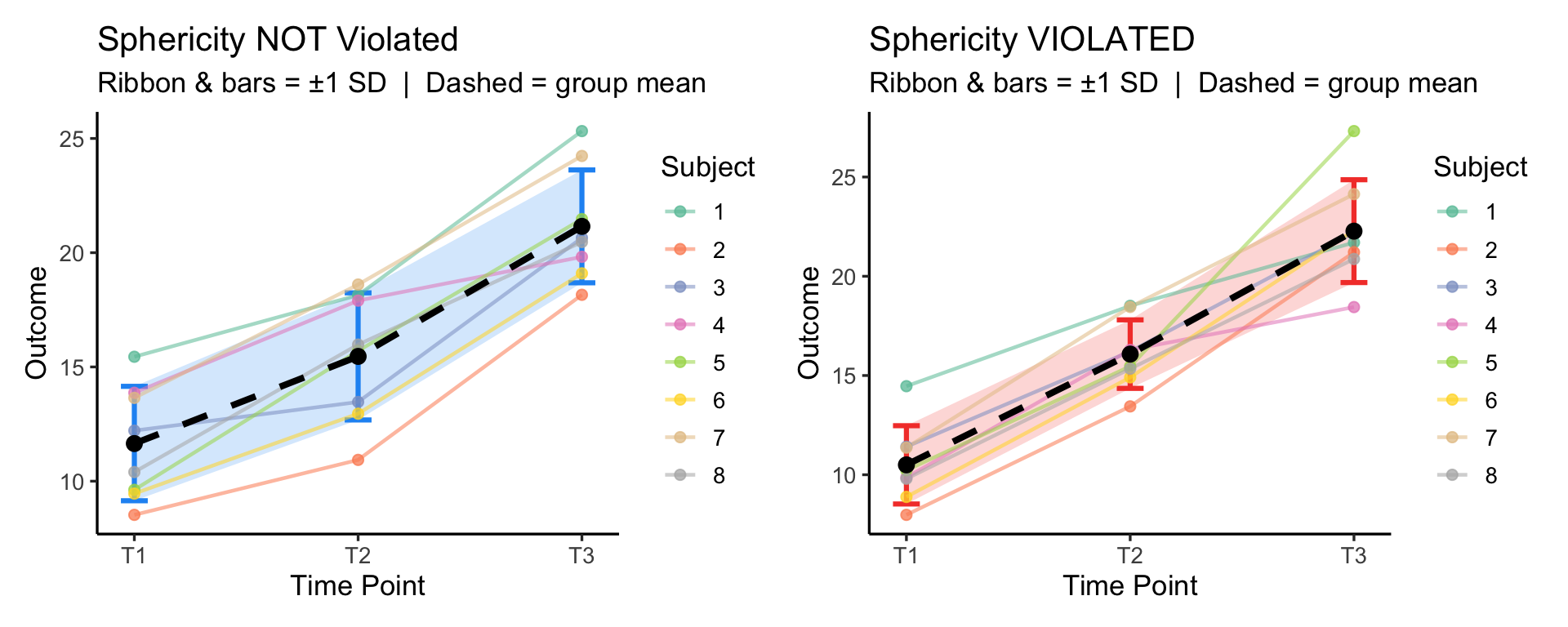
Key intuition:
car::Anova() with summary(result, multivariate = FALSE) directly exposes between-subject variability in its output. Each row in the univariate summary contains both the effect SS and its corresponding Error SS — the error term for that stratum:
| Row in output | Effect SS | Error SS | What it is |
|---|---|---|---|
(Intercept) |
grand mean effect | SS_subjects | Between-subjects variability |
Time |
time effect | SS_error | Within-subjects error |
car::Anova()library(car)
# Use the main case study (4 time points) to match hand-calculated values
dat_wide_main <- tribble(
~ID, ~time1, ~time2, ~time3, ~time4,
1, 10, 16, 25, 26,
2, 12, 19, 27, 25,
3, 13, 20, 28, 28,
4, 12, 18, 25, 15,
5, 11, 20, 26, 18,
6, 10, 22, 27, 19
)
resp <- dat_wide_main |> select(time1, time2, time3, time4) |> as.matrix()
mlm <- lm(resp ~ 1)
idata <- data.frame(Time = factor(paste0("time", 1:4)))
result <- Anova(mlm, idata = idata, idesign = ~Time, type = "III")
summary(result, multivariate = FALSE)
Univariate Type III Repeated-Measures ANOVA Assuming Sphericity

            Sum Sq num Df Error SS den Df F value    Pr(>F)
(Intercept) 9282.7      1   54.333      5 854.233 8.789e-07 ***
Time         713.0      3  116.000     15  30.733 1.192e-06 ***
---
Signif. codes:  0 '***' 0.001 '**' 0.01 '*' 0.05 '.' 0.1 ' ' 1


Mauchly Tests for Sphericity

     Test statistic    p-value
Time        0.00128 0.00025656


Greenhouse-Geisser and Huynh-Feldt Corrections
 for Departure from Sphericity

      GG eps Pr(>F[GG])
Time 0.40219   0.001161 **
---
Signif. codes:  0 '***' 0.001 '**' 0.01 '*' 0.05 '.' 0.1 ' ' 1

        HF eps  Pr(>F[HF])
Time 0.4603901 0.000586618
The Error SS on the (Intercept) row = SS_{subjects} (between-subject variability). The Error SS on the Time row = SS_{error} (within-subject error used in F-test).
uni <- summary(result, multivariate = FALSE)$univariate.tests

# Between-subjects SS = error SS of the intercept stratum
SS_between_subjects <- uni["(Intercept)", "Error SS"]

# Within-subjects error SS = error SS of the Time effect
SS_within_error <- uni["Time", "Error SS"]

cat("SS_between_subjects =", round(SS_between_subjects, 3), "\n")  # expect 54.33
SS_between_subjects = 54.333 cat("SS_within_error =", round(SS_within_error, 3), "\n") # expect 116.00SS_within_error = 116 | Component | Available from car::Anova() |
How to Obtain |
|---|---|---|
| Between-subjects | ✅ Yes | uni["(Intercept)", "Error SS"] |
| Within-subjects error | ✅ Yes | uni["Time", "Error SS"] |
Recall the original study: six dogs, histamine measured at four time points after drug injection. Now suppose the six dogs were randomly assigned to two groups before the study began:
Discussion question: How does adding a between-subjects group factor change the analysis? What new effects can we now test?
library(tidyverse)

dat_mixed <- tribble(
  ~ID, ~Group,       ~time1, ~time2, ~time3, ~time4,
  1,   "Control",    10,     16,     25,     26,
  2,   "Control",    12,     19,     27,     25,
  3,   "Control",    13,     20,     28,     28,
  4,   "Treatment",  12,     18,     25,     15,
  5,   "Treatment",  11,     20,     26,     18,
  6,   "Treatment",  10,     22,     27,     19
) |>
  mutate(ID = factor(ID), Group = factor(Group))

dat_mixed_long <- dat_mixed |>
  pivot_longer(starts_with("time"), names_to = "Time", values_to = "Y") |>
  mutate(Time = factor(Time, levels = paste0("time", 1:4)),
         Time_num = as.integer(Time))

dat_mixed_long
# A tibble: 24 × 5
ID Group Time Y Time_num
<fct> <fct> <fct> <dbl> <int>
1 1 Control time1 10 1
2 1 Control time2 16 2
3 1 Control time3 25 3
4 1 Control time4 26 4
5 2 Control time1 12 1
6 2 Control time2 19 2
7 2 Control time3 27 3
8 2 Control time4 25 4
9 3 Control time1 13 1
10 3 Control time2 20 2
# ℹ 14 more rowslibrary(patchwork)
group_means <- dat_mixed_long |>
group_by(Group, Time, Time_num) |>
summarise(mean_Y = mean(Y), sd_Y = sd(Y), .groups = "drop")
# Individual trajectories + group mean ribbons
p_mixed <- ggplot(dat_mixed_long, aes(x = Time_num, y = Y)) +
geom_ribbon(
data = group_means,
aes(x = Time_num, y = mean_Y,
ymin = mean_Y - sd_Y, ymax = mean_Y + sd_Y,
fill = Group, group = Group),
alpha = 0.15, inherit.aes = FALSE
) +
geom_line(aes(group = ID, color = Group), alpha = 0.5, linewidth = 0.8) +
geom_point(aes(color = Group), size = 2, alpha = 0.8) +
geom_line(
data = group_means,
aes(x = Time_num, y = mean_Y, color = Group, group = Group),
linewidth = 1.5, linetype = "dashed", inherit.aes = FALSE
) +
geom_point(
data = group_means,
aes(x = Time_num, y = mean_Y, color = Group),
size = 3.5, inherit.aes = FALSE
) +
scale_x_continuous(breaks = 1:4,
labels = paste0("time", 1:4)) +
scale_color_manual(values = c(Control = "#2196F3", Treatment = "#F44336")) +
scale_fill_manual(values = c(Control = "#2196F3", Treatment = "#F44336")) +
labs(
title = "Histamine Over Time by Group",
subtitle = "Ribbon = ±1 SD | Dashed = group mean trajectory",
x = "Time Point", y = "Histamine Concentration",
color = "Group", fill = "Group"
) +
theme_classic(base_size = 13)
p_mixed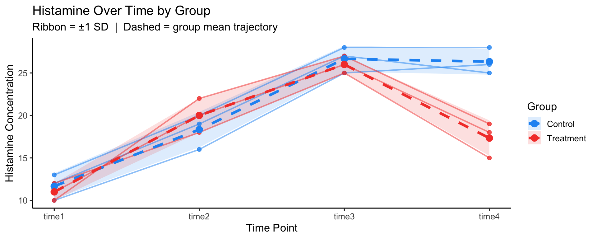
Before reading ahead — what effects should we test?
This is a Mixed Design (Split-Plot) ANOVA — it combines:
| Factor | Type | Levels |
|---|---|---|
| Group | Between-subjects | Control, Treatment |
| Time | Within-subjects | time1, time2, time3, time4 |
Three effects can now be tested:
In R:
model_mixed <- aov(Y ~ Group * Time + Error(ID/Time), data = dat_mixed_long)
summary(model_mixed)
Error: ID
          Df Sum Sq Mean Sq F value Pr(>F)
Group      1  28.17  28.167   4.306  0.107
Residuals  4  26.17   6.542

Error: ID:Time
           Df Sum Sq Mean Sq F value   Pr(>F)
Time        3  713.0  237.67  166.14 4.90e-10 ***
Group:Time  3   98.8   32.94   23.03 2.88e-05 ***
Residuals  12   17.2    1.43
---
Signif. codes:  0 '***' 0.001 '**' 0.01 '*' 0.05 '.' 0.1 ' ' 1
Group is tested against the between-subjects error (MS among dogs within groups)Time and Group:Time are tested against the within-subjects error (MS of residuals after removing dog and time effects)Looking at the plot: the two group means diverge at time4 — control dogs maintain high histamine while treatment dogs drop back. This crossing/diverging pattern is a visual cue for a potential Group × Time interaction, suggesting the drug suppresses the late-phase histamine response.
In the original study, all four time points are passive measurements after a single injection. But now suppose time3 is not a measurement — it is when the intervention (drug injection) occurs:
Discussion question: How does treating time3 as an intervention point change how we interpret the data and what comparisons matter most?
The within-subjects factor Time now has a qualitative break — the first two time points are a pre-intervention baseline and the last is a post-intervention outcome. Simply testing a main effect of Time conflates the baseline trend with the intervention effect.
A more targeted analysis would compare:
| Contrast | Formula | Question |
|---|---|---|
| Pre-trend | time3 − time1 | Was histamine already rising across the baseline period? |
| Intervention effect | time4 − time3 | Did histamine change immediately after the injection session? |
| DiD | (time4 − time3) − (time3 − time1) | Does the post-injection change exceed the natural pre-trend? |
library(tidyverse)

dat_intervention <- tribble(
  ~ID, ~time1, ~time2, ~time3, ~time4,
  1,   10,     16,     25,     26,
  2,   12,     19,     27,     25,
  3,   13,     20,     28,     28,
  4,   12,     18,     25,     15,
  5,   11,     20,     26,     18,
  6,   10,     22,     27,     19
) |>
  pivot_longer(starts_with("time"), names_to = "Time", values_to = "Y") |>
  mutate(Time = factor(Time, levels = paste0("time", 1:4)),
         Time_num = as.integer(Time),
         Phase = case_when(
           Time_num <= 2 ~ "Pre-Intervention",
           Time_num == 3 ~ "Intervention",
           Time_num == 4 ~ "Post-Intervention"
         ) |> factor(levels = c("Pre-Intervention", "Intervention", "Post-Intervention")),
         ID = factor(ID))

means_int <- dat_intervention |>
  group_by(Time, Time_num) |>
  summarise(mean_Y = mean(Y), .groups = "drop")

ggplot(dat_intervention, aes(x = Time_num, y = Y)) +
  # Shade the intervention time point
  annotate("rect", xmin = 2.5, xmax = 3.5, ymin = -Inf, ymax = Inf,
           fill = "#FF9800", alpha = 0.15) +
  annotate("text", x = 3, y = 30, label = "Intervention", color = "#E65100",
           size = 3.5, fontface = "bold") +
  geom_line(aes(group = ID, color = ID), alpha = 0.5, linewidth = 0.8) +
  geom_point(aes(color = ID), size = 2.5, alpha = 0.8) +
  geom_line(data = means_int, aes(x = Time_num, y = mean_Y, group = 1),
            color = "black", linewidth = 1.5, linetype = "dashed",
            inherit.aes = FALSE) +
  geom_point(data = means_int, aes(x = Time_num, y = mean_Y),
             color = "black", size = 3.5, inherit.aes = FALSE) +
  scale_x_continuous(breaks = 1:4, labels = paste0("time", 1:4)) +
  scale_color_brewer(palette = "Set2") +
  labs(title = "Histamine Trajectory with Intervention at time3",
       subtitle = "Shaded region = intervention session  |  Dashed = group mean",
       x = "Time Point", y = "Histamine Concentration", color = "Dog") +
  theme_classic(base_size = 13)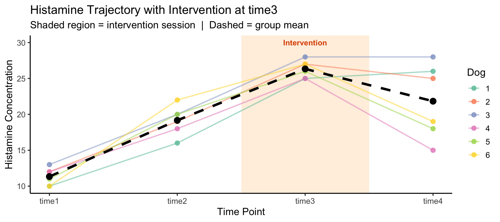
Before reading — how would you re-frame the hypothesis tests given this design?
The key shift: time3 should not be treated as just another within-subjects level — it marks a design boundary between baseline and outcome phases.
Recommended approach — planned contrasts instead of omnibus F:
library(tidyverse)

# Compute the two key contrasts per dog
contrasts_df <- dat_intervention |>
  select(ID, Time, Y) |>
  pivot_wider(names_from = Time, values_from = Y) |>
  mutate(
    pre_trend           = time3 - time1,  # baseline drift up to intervention
    intervention_effect = time4 - time3,  # post vs intervention session
    did                 = intervention_effect - pre_trend  # difference-in-differences
  )

contrasts_df |> select(ID, pre_trend, intervention_effect, did)
# A tibble: 6 × 4
ID pre_trend intervention_effect did
<fct> <dbl> <dbl> <dbl>
1 1 15 1 -14
2 2 15 -2 -17
3 3 15 0 -15
4 4 13 -10 -23
5 5 15 -8 -23
6 6 17 -8 -25Test 1 — Is the pre-intervention trend significantly different from zero?
t.test(contrasts_df$pre_trend, mu = 0)
    One Sample t-test

data:  contrasts_df$pre_trend
t = 29.047, df = 5, p-value = 9.063e-07
alternative hypothesis: true mean is not equal to 0
95 percent confidence interval:
 13.67256 16.32744
sample estimates:
mean of x
       15
Test 2 — Is there a significant intervention effect (time4 vs time3)?
t.test(contrasts_df$intervention_effect, mu = 0)
    One Sample t-test

data:  contrasts_df$intervention_effect
t = -2.3342, df = 5, p-value = 0.06686
alternative hypothesis: true mean is not equal to 0
95 percent confidence interval:
 -9.4557369  0.4557369
sample estimates:
mean of x
     -4.5
Test 3 — Difference-in-differences: does the intervention effect exceed the pre-trend?
t.test(contrasts_df$did, mu = 0)
    One Sample t-test

data:  contrasts_df$did
t = -10.115, df = 5, p-value = 0.0001618
alternative hypothesis: true mean is not equal to 0
95 percent confidence interval:
 -24.45574 -14.54426
sample estimates:
mean of x
    -19.5
Visualise the contrasts per dog:
contrasts_df |>
  select(ID, pre_trend, intervention_effect, did) |>
  pivot_longer(-ID, names_to = "Contrast", values_to = "Value") |>
  mutate(Contrast = factor(Contrast,
    levels = c("pre_trend", "intervention_effect", "did"),
    labels = c("Pre-trend\n(time3 − time1)",
               "Intervention effect\n(time4 − time3)",
               "DiD\n(effect − trend)"))) |>
  ggplot(aes(x = Contrast, y = Value, color = ID, group = ID)) +
  geom_hline(yintercept = 0, linetype = "dashed", color = "grey50") +
  geom_line(alpha = 0.4, linewidth = 0.8) +
  geom_point(size = 3) +
  stat_summary(aes(group = 1), fun = mean, geom = "point",
               shape = 18, size = 5, color = "black") +
  stat_summary(aes(group = 1), fun = mean, geom = "line",
               linewidth = 1.2, color = "black", linetype = "dashed") +
  scale_color_brewer(palette = "Set2") +
  labs(title = "Planned Contrasts per Dog",
       subtitle = "Diamond = group mean  |  Dashed line at zero = no effect",
       x = NULL, y = "Contrast Value", color = "Dog") +
  theme_classic(base_size = 13)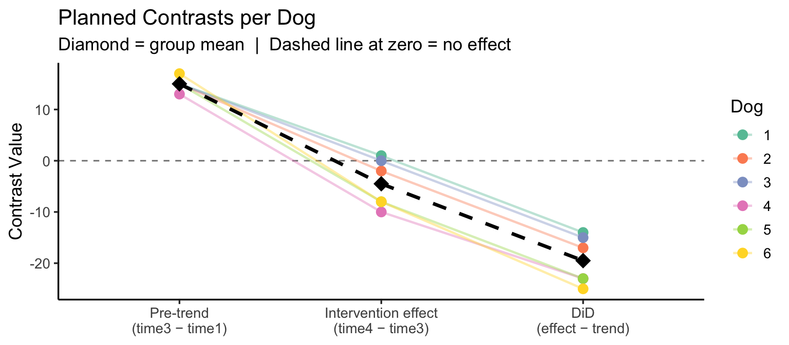
Interpretation: