# install.packages("moments")
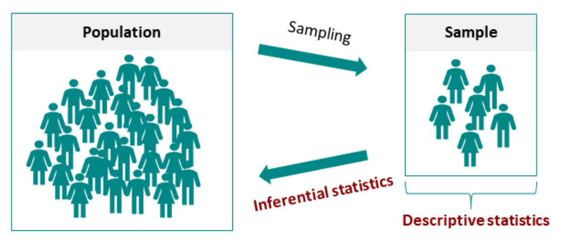
moments::skewness(c(1:10, 100))[1] 2.793716moments::skewness(rnorm(100, 0, 1)) # should be close to 0[1] -0.1416608Statistics can be classified by purpose:
# install.packages("moments")
moments::skewness(c(1:10, 100))[1] 2.793716moments::skewness(rnorm(100, 0, 1)) # should be close to 0[1] -0.1416608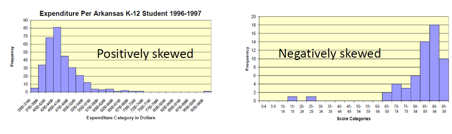
set.seed(1234)
# Simulate a skewed normal distribution using beta distribution
neg_skewed_data <- rbeta(10000,5,2)
hist(neg_skewed_data, main = "Negative Skewed Distribution")
pos_skewed_data <- rbeta(10000,2,5)
hist(pos_skewed_data, main = "Positive Skewed Distribution")
library(ggplot2)
library(tidyr)
data.frame(
  neg = neg_skewed_data,
  pos = pos_skewed_data
  ) |>
  pivot_longer(c(neg, pos), names_to = "Type") |>
  ggplot(aes(y = value, fill = Type)) +
  geom_boxplot() +
  scale_fill_discrete(labels = c("Negative Skewed", "Positive Skewed"), name = "")
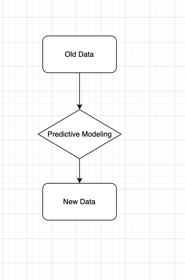
Definition: Use observed data to produce the most accurate prediction possible for new data. Here, the primary goal is that the predicted values have the highest possible fidelity to the true value of the new data.
Example: A simple example would be for a book buyer to predict how many copies of a particular book should be shipped to their store for the next month.
How many houses burned in California wildfire in the first week?
Which factor is most important causing the fires?
How likely the California wildfire will not happen again in next 5 years?
How likely human will live on Mars?
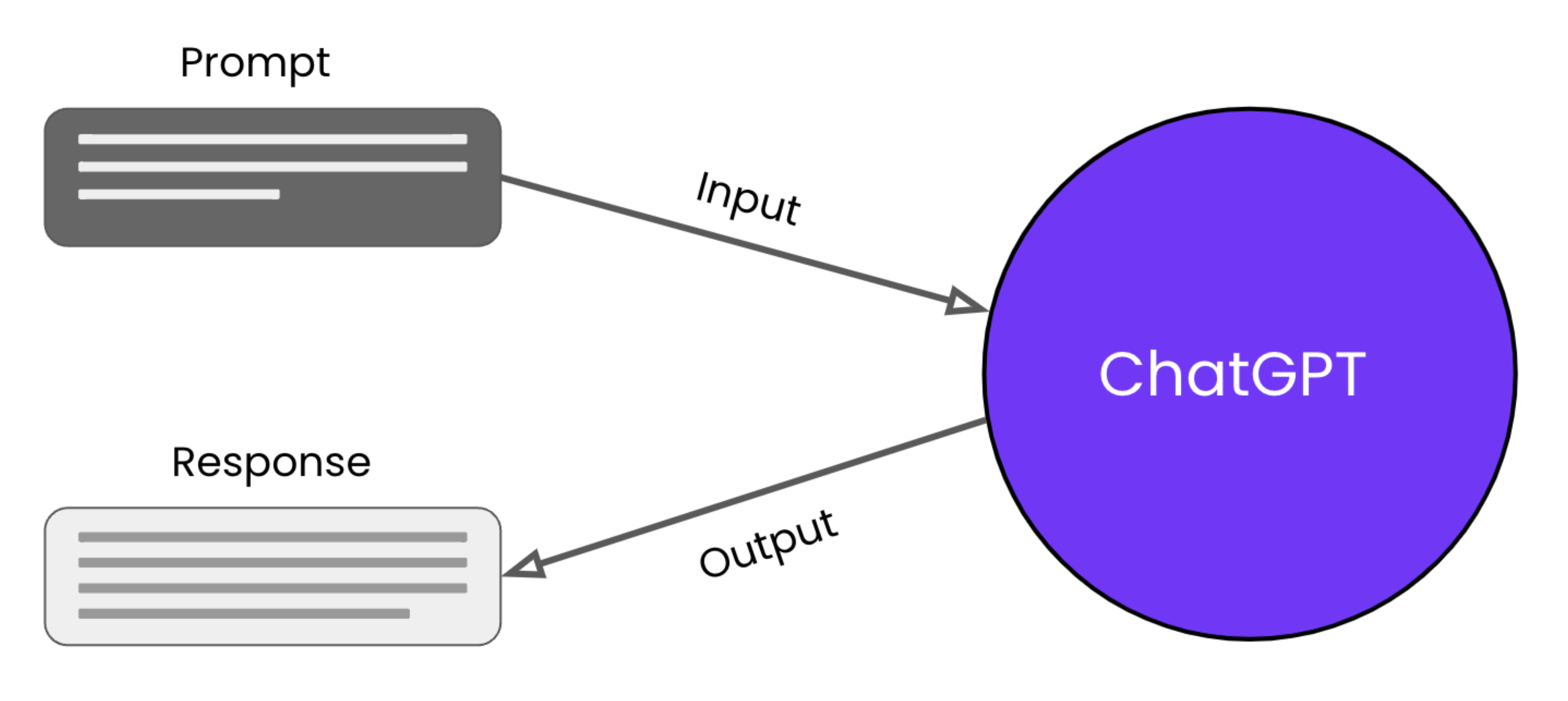
Which type of statistics is used by ChatGPT?
Steps for Inferential Statistical Testing:
One-Way ANOVA
Purpose: Tests one factor with three or more levels on a continuous outcome.
Use Case: Comparing means across multiple groups (e.g., diet types on weight loss).
Two-Way ANOVA
Purpose: Examines two factors and their interaction on a continuous outcome.
Use Case: Studying effects of diet and exercise on weight loss.
Repeated Measures ANOVA
Purpose: Tests the same subjects under different conditions or time points.
Use Case: Longitudinal studies measuring the same outcome over time (e.g., cognitive tests after varying sleep durations).
Mixed-Design ANOVA
Purpose: Combines between-subjects and within-subjects factors in one analysis.
Use Case: Evaluating treatment effects over time with control and experimental groups.
Multivariate Analysis of Variance (MANOVA)
Purpose: Assesses multiple continuous outcomes (dependent variables) influenced by independent variables.
Use Case: Impact of psychological interventions on anxiety, stress, and self-esteem.
party: Political affiliationscores: Attitude scores for survey respondents## Install the package ESRM64103 from GitHub
remotes::install_github("JihongZ/ESRM64103")library(ESRM64103)
library(dplyr)
exp_political_attitude party scores
1 Democrat 4
2 Democrat 3
3 Democrat 5
4 Democrat 4
5 Democrat 4
6 Republican 6
7 Republican 5
8 Republican 3
9 Republican 7
10 Republican 4
11 Republican 5
12 Independent 8
13 Independent 9
14 Independent 8
15 Independent 7
16 Independent 8
Calculate mean, standard deviation, and variance for each political group
Grand mean across all groups: 5.625
# Grand mean
mean(exp_political_attitude$scores)[1] 5.625exp_political_attitude$party <- factor(exp_political_attitude$party,
levels = c("Democrat", "Republican", "Independent"))
mean_byGroup <- exp_political_attitude |>
group_by(party) |>
summarise(Mean = mean(scores),
SD = round(sd(scores), 2),
Vars = round(var(scores), 2),
N = n())
mean_byGroup# A tibble: 3 × 5
party Mean SD Vars N
<fct> <dbl> <dbl> <dbl> <int>
1 Democrat 4 0.71 0.5 5
2 Republican 5 1.41 2 6
3 Independent 8 0.71 0.5 5library(ggplot2)
ggplot(data = mean_byGroup) +
geom_bar(mapping = aes(x = party, y = Mean, fill = party), stat = "identity", width = .5) +
geom_label(aes(x = party, y = Mean, label = Mean), nudge_y = .3) +
labs(title = "Attitudes Toward the Tax Return") +
theme(text = element_text(size = 15))
In research, we often need to compute descriptive statistics for multiple continuous variables simultaneously. Here are several approaches:
# Generate simulated student performance data
set.seed(2025)
n_students <- 100
student_data <- data.frame(
student_id = 1:n_students,
math_score = rnorm(n_students, mean = 75, sd = 12),
reading_score = rnorm(n_students, mean = 78, sd = 10),
science_score = rnorm(n_students, mean = 72, sd = 11),
study_hours = rgamma(n_students, shape = 2, scale = 3),
attendance_rate = rbeta(n_students, shape1 = 8, shape2 = 2) * 100
)sapply()# Select only continuous variables
continuous_vars <- student_data[, c("math_score", "reading_score", "science_score", "study_hours", "attendance_rate")]
# Compute mean, sd, and range for each variable
desc_stats <- data.frame(
Mean = sapply(continuous_vars, mean),
SD = sapply(continuous_vars, sd),
Min = sapply(continuous_vars, min),
Max = sapply(continuous_vars, max),
Range = sapply(continuous_vars, function(x) max(x) - min(x))
)
round(desc_stats, 2) Mean SD Min Max Range
math_score 74.94 12.24 45.59 109.23 63.64
reading_score 78.09 9.65 58.84 100.50 41.66
science_score 72.10 10.83 40.66 99.39 58.73
study_hours 6.03 4.81 0.40 26.14 25.74
attendance_rate 80.53 10.53 49.08 99.10 50.02dplyr package with across()library(dplyr)
student_data |>
summarise(
across(
c(math_score, reading_score, science_score, study_hours, attendance_rate),
list(
Mean = ~mean(.x),
SD = ~sd(.x),
Min = ~min(.x),
Max = ~max(.x),
Range = ~max(.x) - min(.x)
),
.names = "{.col}_{.fn}"
)
) |>
tidyr::pivot_longer(
everything(),
names_to = c("Variable", "Statistic"),
names_sep = "_(?=[^_]+$)",
values_to = "Value"
) |>
tidyr::pivot_wider(
names_from = Statistic,
values_from = Value
) |>
mutate(across(where(is.numeric), ~round(.x, 2)))# A tibble: 5 × 6
Variable Mean SD Min Max Range
<chr> <dbl> <dbl> <dbl> <dbl> <dbl>
1 math_score 74.9 12.2 45.6 109. 63.6
2 reading_score 78.1 9.65 58.8 100. 41.7
3 science_score 72.1 10.8 40.7 99.4 58.7
4 study_hours 6.03 4.81 0.4 26.1 25.7
5 attendance_rate 80.5 10.5 49.1 99.1 50.0psych::describe()The psych package provides a comprehensive describe() function:
library(psych)
continuous_vars |>
describe() |>
select(n, mean, sd, min, max, range) |>
round(2) n mean sd min max range
math_score 100 74.94 12.24 45.59 109.23 63.64
reading_score 100 78.09 9.65 58.84 100.50 41.66
science_score 100 72.10 10.83 40.66 99.39 58.73
study_hours 100 6.03 4.81 0.40 26.14 25.74
attendance_rate 100 80.53 10.53 49.08 99.10 50.02You can also compute descriptives by groups:
# Add a grouping variable
student_data$program <- sample(c("STEM", "Arts", "Social Sciences"),
n_students, replace = TRUE,
prob = c(0.4, 0.3, 0.3))# Compute descriptives by program
student_data |>
group_by(program) |>
summarise(
N = n(),
Math_Mean = mean(math_score),
Math_SD = sd(math_score),
Reading_Mean = mean(reading_score),
Reading_SD = sd(reading_score),
Science_Mean = mean(science_score),
Science_SD = sd(science_score)
) |>
mutate(across(where(is.numeric) & !N, ~round(.x, 2)))# A tibble: 3 × 8
program N Math_Mean Math_SD Reading_Mean Reading_SD Science_Mean
<chr> <int> <dbl> <dbl> <dbl> <dbl> <dbl>
1 Arts 30 74.2 12.7 80.5 10.1 72.8
2 STEM 44 74.3 12.4 77.6 9.1 73.4
3 Social Sciences 26 76.9 11.7 76.1 9.8 69.2
# ℹ 1 more variable: Science_SD <dbl>remotes::install_github("JihongZ/ESRM64103")
library(ESRM64103)
library(dplyr)
exp_political_attitude
exp_political_attitude$party <- factor(exp_political_attitude$party,
                                       levels = c("Democrat", "Republican", "Independent"))
mean_byGroup <- exp_political_attitude |>
  group_by(party) |>
  summarise(Mean = mean(scores),
            SD = round(sd(scores), 2),
            Vars = round(var(scores), 2),
            N = n())
mean_byGroup
anova_model <- lm(scores ~ party, data = exp_political_attitude)
anova(anova_model)
State the null hypothesis and alternative hypothesis:
Set the significant alpha = 0.05
Calculate Observed F-statistics:
F_{obs} = \frac{SS_b/df_b}{SS_w/df_w}
Degrees of freedom: df_b = 3 (groups) - 1 = 2, df_w = 16 (samples) - 3 (groups) = 13
Between-group sum of squares: SS_b = \sum_{j=1}^{g} n_j(\bar{Y}_j - \bar{Y})^2 = 43.75 where n_j is group sample size, \bar{Y}_j is group mean, and \bar{Y} is the grand mean.
Within-group sum of squares: SS_w = \sum_{j=1}^{3} \sum_{i=1}^{n_j}(Y_{ij}-\bar{Y}_j)^2 = 14.00 where Y_{ij} is individual i’s score in group j.
GrandMean <- mean(exp_political_attitude$scores)
## Between-group Sum of Squares
cat("Between-group Sum of Squares: ", sum(mean_byGroup$N * (mean_byGroup$Mean - GrandMean)^2))
Between-group Sum of Squares: 43.75## Within-group Sum of Squares
SSw_dt <- exp_political_attitude |>
group_by(party) |>
mutate(GroupMean = mean(scores),
Diff_sq = (scores - GroupMean)^2)
cat("Within-group Sum of Squares: ", sum(SSw_dt$Diff_sq))Within-group Sum of Squares: 14SS_b <- sum(mean_byGroup$N * (mean_byGroup$Mean - GrandMean)^2)
SS_w <- sum(SSw_dt$Diff_sq)
df_b = 2
df_w = 16 - 3
F_bw = (SS_b / df_b) / (SS_w / df_w)anova_model <- lm(scores ~ party, data = exp_political_attitude)
anova(anova_model)Analysis of Variance Table
Response: scores
Df Sum Sq Mean Sq F value Pr(>F)
party 2 43.75 21.8750 20.312 9.994e-05 ***
Residuals 13 14.00 1.0769
---
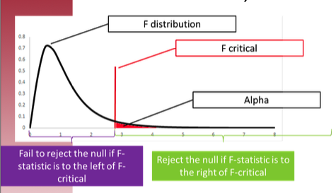
Signif. codes: 0 '***' 0.001 '**' 0.01 '*' 0.05 '.' 0.1 ' ' 1Results show rejection of H_0 (F_{obs} > F_{critical})
F-statistic has two degree of freedoms (df = 2). This is the density distribution of F-statistics for degree of freedoms as 2 and 13.
# Set degrees of freedom for the numerator and denominator
num_df <- 2  # Change this as per your specification
den_df <- 13  # Change this as per your specification

# Generate a sequence of F values
f_values <- seq(0, 8, length.out = 1000)

# Calculate the density of the F-distribution
f_density <- df(f_values, df1 = num_df, df2 = den_df)

# Create a data frame for plotting
data_to_plot <- data.frame(F_Values = f_values, Density = f_density)
data_to_plot$Reject05 <- data_to_plot$F_Values > 3.81
data_to_plot$Reject01 <- data_to_plot$F_Values > 6.70
# Plot the density using ggplot2
ggplot(data_to_plot) +
  geom_area(aes(x = F_Values, y = Density), fill = "grey",
            data = filter(data_to_plot, !Reject05)) + # Draw the line
  geom_area(aes(x = F_Values, y = Density), fill = "yellow",
            data = filter(data_to_plot, Reject05)) + # Draw the line
  geom_area(aes(x = F_Values, y = Density), fill = "tomato",
            data = filter(data_to_plot, Reject01)) + # Draw the line
  geom_vline(xintercept = 3.81, linetype = "dashed", color = "red") +
  geom_label(label = "F_crit = 3.81 (alpha = .05)", x = 3.81, y = .5, color = "red") +
  geom_vline(xintercept = 6.70, linetype = "dashed", color = "royalblue") +
  geom_label(label = "F_crit = 6.70 (alpha = .01)", x = 6.70, y = .5, color = "royalblue") +
  ggtitle("Density of F-Distribution") +
  xlab("F values") +
  ylab("Density") +
  theme_classic()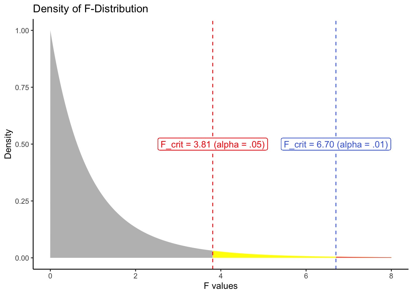
Set the alpha \alpha (i.e., type I error rate)—rejection rate vs. p-value
Alpha determines several values for statistical hypothesis testing: the critical value of the test statistics, the rejection region, etc.
Large sample sizes typically use lower alpha levels: .01 or .001 (more restrictive rejection rate)
When we conduct hypothesis testing, four possible outcomes can occur:
| Reality | ||
| Decision | H_0 is true | H_0 is false |
| Fail to reject H_0 | Correct Decision | Error made. Type II error (\beta). |
| Reject H_0 | Error made. Type I error (\alpha) |
Correct Decision (Power) |
Investigate where the variability in the outcome comes from.
In this study: Do people’s attitude scores differ because of their political party affiliation?
When we have factors influencing the outcome, the total variability can be decomposed as follows:
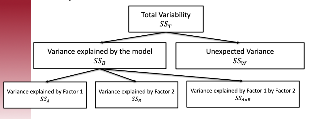
Core idea: Comparing the variances between groups and within groups to ascertain if the means of different groups are significantly different from each other.
Logic: If the between-group variance (due to systematic differences caused by the independent variable) is significantly greater than the within-group variance (attributable to random error), the observed differences between group means are likely not due to chance.
F-statistics formula for one-way ANOVA:
F_{obs} = \frac{SS_{between}/df_{between}}{SS_{within}/df_{within}}
A one-way ANOVA was conducted to compare the level of concern for tax reform among three political groups: Democrats, Republicans, and Independents. There was a significant effect of political affiliation on tax reform concern at the p < .001 level for the three conditions [F(2, 13) = 20.31, p < .001]. This result indicates significant differences in attitudes toward tax reform among the groups.
P-values: The probability of observing data as extreme as, or more extreme than, the data observed under the assumption that the null hypothesis is true.
The lower the p-value, the less likely we would see the observed data given the null hypothesis is true
Question: Given that we already have the observed data, does a lower p-value mean the null hypothesis is unlikely to be true?
Answer: No. P(\text{observed data} | H_0 = \text{true}) \neq P(H_0 = \text{true} | \text{observed data}). P-values are often misconstrued as the probability that the null hypothesis is true given the observed data. However, this interpretation is incorrect.
Type I error, also known as a “false positive,” occurs when the null hypothesis is incorrectly rejected when it is, in fact, true.
The alpha level \alpha set before conducting a test (commonly \alpha = 0.05) defines the cutoff point for the p-value below which the null hypothesis will be rejected.
A p-value less than the alpha level suggests a low probability that the observed data would occur if the null hypothesis were true. Consequently, rejecting the null hypothesis in this context implies there is a statistically significant difference likely not due to random chance.
If you set up a high alpha level (0.1), you are more likely to have p-value lower than alpha, which means you are more likely reject the null hypothesis that may be true, which means you may make Type 1 error.
If you set up a low alpha level (0.001), you are less likely to have p-value lower than alpha, which means you are more likely retain the null hypothesis that may be false, which means you may make Type 2 error.
Relying solely on p-values to reject the null hypothesis can be problematic for several reasons:
Binary Decision Making: The use of a threshold (e.g., \alpha = 0.05) to determine whether to reject the null hypothesis reduces the complexity of the data to a binary decision. This can oversimplify the interpretation and overlook nuances in the data.
Neglect of Effect Size: P-values do not convey the size or practical importance of an effect. A very small effect can produce a small p-value if the sample size is large enough, leading to rejection of the null hypothesis even when the effect may not be practically significant.
Probability of Extremes Under the Null: Since p-values quantify the extremeness of the observed data under the null hypothesis, they do not address whether similarly extreme data could also occur under alternative hypotheses. This can lead to an overemphasis on the null hypothesis and potentially disregard other plausible explanations for the data.
A study investigates the effect of different sleep durations on the academic performance of university students. Three groups are defined based on nightly sleep duration: Less than 6 hours, 6 to 8 hours, and more than 8 hours.
We can simulate the data
# Set seed for reproducibility
set.seed(42)

# Generate data for three sleep groups
less_than_6_hours <- rnorm(30, mean = 65, sd = 10)
six_to_eight_hours <- rnorm(50, mean = 75, sd = 8)
more_than_8_hours <- rnorm(20, mean = 78, sd = 7)

# Combine data into a single data frame
sleep_data <- data.frame(
  Sleep_Group = factor(c(rep("<6 hours", 30), rep("6-8 hours", 50), rep(">8 hours", 20))),
  Exam_Score = c(less_than_6_hours, six_to_eight_hours, more_than_8_hours)
)

# View the first few rows of the dataset
head(sleep_data)
Sleep_Group Exam_Score
1 <6 hours 78.70958
2 <6 hours 59.35302
3 <6 hours 68.63128
4 <6 hours 71.32863
5 <6 hours 69.04268
6 <6 hours 63.93875## There are two columns: (1) Sleep_Group (Group variable, IV) (2) Exam_Score (Outcome, DV)
mod <- lm(Exam_Score ~ Sleep_Group, data = sleep_data)
mod_aov <- aov(mod)
summary(mod_aov) # F-value = 14.15, p < .05 Df Sum Sq Mean Sq F value Pr(>F)
Sleep_Group 2 2411 1205.4 14.15 4.06e-06 ***
Residuals 97 8264 85.2
---
Signif. codes: 0 '***' 0.001 '**' 0.01 '*' 0.05 '.' 0.1 ' ' 1Groups:
Less than 6 hours: 30 students
6 to 8 hours: 50 students
More than 8 hours: 20 students
Performance Metric: Average exam scores out of 100.
Less than 6 hours: Mean = 65, SD = 10
6 to 8 hours: Mean = 75, SD = 8
More than 8 hours: Mean = 78, SD = 7
Analysis: One-way ANOVA was conducted to compare the average exam scores among the three groups.
Results: F_{observed} = [Calculate from your analysis], p = [Report p-value]
Alpha Level: \alpha = 0.05
P-value Interpretation: Compare your p-value to alpha and interpret the result
Conclusion: Based on the results, what can you conclude about the effect of sleep duration on academic performance?
Due on next Tuesday Noon. Here is the google form link.