Make Friends With R, RStudio, Positron, and Quarto

Author

Jihong Zhang

Make Friends With R, RStudio, Positron, and Quarto

Welcome to your first steps in applied multivariate statistics! In this tutorial, you’ll learn how to use R, RStudio, Positron, and Quarto (.qmd files) to run R code, analyze data, and create reproducible reports.


1. What are R, RStudio, Positron, and Quarto?

  • R (required): A powerful programming language for statistical computing and graphics.
  • Quarto (required): A next-generation tool for creating dynamic documents, presentations, and websites with R (and other languages). Quarto files use the .qmd extension. Download link
  • RStudio (optional): An integrated development environment (IDE) that makes using R easier. Download link
  • Positron (optional): A next-generation data science IDE created by Posit (formerly RStudio), built on VS Code architecture, designed for both R and Python workflows. Download link

Choose RStudio or Positron based on your preference


1.4. Getting Started with RStudio: The Classic R IDE

RStudio is the most widely-used IDE for R programming, offering a user-friendly interface that has helped millions of data scientists learn R. It’s mature, stable, and specifically designed for R workflows.

Key Features of RStudio:

  • R-focused design: Built specifically for R programming and statistical analysis
  • Four-panel layout: Organized interface with Source, Console, Environment, and Files/Plots panels
  • Package management: Easy package installation and loading through GUI
  • Project management: RStudio Projects for organized, reproducible workflows
  • Git integration: Built-in version control support
  • R Markdown/Quarto support: Native support for literate programming

RStudio Interface Layout:

  • Source Editor (top-left): Edit .R, .qmd, and other files with syntax highlighting
  • Console (bottom-left): Interactive R console for running commands
  • Environment/History (top-right): View objects, variables, and command history
  • Files/Plots/Packages/Help (bottom-right): Navigate files, view plots, manage packages, access help

Getting Started with RStudio:

  1. Download: Get RStudio Desktop from posit.co/download/rstudio-desktop/
  2. Create projects: Use File → New Project for organized workflows
  3. Customize layout: Tools → Global Options → Pane Layout to adjust panels
  4. Install packages: Use Tools → Install Packages or the Packages panel

Essential RStudio Features:

  • Code completion: Tab completion for functions and variables
  • Help integration: F1 on functions for instant help
  • Object inspector: Click objects in Environment to view details
  • Plot history: Navigate through previous plots in Plots panel
  • Addins: Extend functionality with community-developed tools

RStudio Keyboard Shortcuts:

  • Run code: Ctrl+Enter (Cmd+Enter on Mac)
  • New R script: Ctrl+Shift+N (Cmd+Shift+N)
  • Render document: Ctrl+Shift+K (Cmd+Shift+K)
  • Insert code chunk: Ctrl+Alt+I (Cmd+Option+I)
  • Go to line: Ctrl+G (Cmd+G)

1.5. Introducing Positron: A Modern Data Science IDE

Positron is Posit’s newest IDE, designed specifically for data scientists working with R and Python. Built on the VS Code platform, it combines the best of modern development tools with data science-specific features.

Key Features of Positron:

  • Multi-language support: Seamlessly work with R and Python in the same environment
  • Interactive console: Enhanced R and Python consoles with rich outputs
  • Variable viewer: Inspect data frames, lists, and objects with interactive exploration
  • Plot viewer: View and interact with ggplot2, matplotlib, and other graphics
  • Integrated terminal: Access system commands and package managers
  • Extension ecosystem: Leverage VS Code’s vast extension library

Positron vs RStudio:

Feature RStudio Positron
Language Support R-focused R + Python
Base Platform Custom Qt VS Code
Extensions Limited Extensive VS Code ecosystem
Performance Traditional Modern, faster startup
Interface Fixed panels Flexible layouts
Learning Curve R-specific General programming

Getting Started with Positron:

  1. Download: Get Positron from positron.posit.co
  2. Open projects: Use File → Open Folder or create new R/Python projects
  3. Run code: Use Ctrl+Enter (Cmd+Enter on Mac) to execute code
  4. Explore data: Click variables in the Variables panel to explore interactively

Positron Keyboard Shortcuts:

  • Run code: Ctrl+Enter (Cmd+Enter)
  • New R console: Ctrl+Shift+`
  • Render Quarto: Ctrl+Shift+K (Cmd+Shift+K)
  • Command palette: Ctrl+Shift+P (Cmd+Shift+P)

1.6. RStudio Basics

  • Source Editor (top-left): edit .R/.qmd files
  • Choose your IDE: Try both RStudio and Positron to see which fits your workflow
  • Explore the tidyverse (readr, dplyr, tidyr, ggplot2)
  • Learn Quarto for documents, slides, and websites
  • If using Positron, explore Python integration for data science
  • Practice by importing a dataset, cleaning it, summarizing, and plottingpackages, read help
  • Useful shortcuts: Run line/selection (Cmd+Enter), Render (Cmd+Shift+K)

1.7. IDE Basics: RStudio vs Positron

RStudio Layout:

  • Source Editor (top-left): edit .R/.qmd files
  • Console/Terminal (bottom-left): run commands
  • Environment/History (top-right): objects and history
  • Files/Plots/Packages/Help (bottom-right): navigate, view plots, manage packages, read help

Positron Layout:

  • Editor: Central area for .R/.qmd files with syntax highlighting
  • Console: Bottom panel with enhanced R/Python consoles
  • Variables: Side panel with interactive data exploration
  • Use projects and here::here() for reliable paths in both RStudio and Positron options
  • Explorer: File browser and project navigation

Common Shortcuts (Both IDEs):

  • Rendering:
    • RStudio: Use the Render button or Cmd+Shift+K
    • Positron: Use Ctrl+Shift+K or the Command Palette
    • Terminal: Run quarto render in any IDE

Note: Both RStudio and Positron support project-based workflows, making it easy to manage paths and dependencies. Render Quarto: Cmd+Shift+K (Mac) / Ctrl+Shift+K (Windows/Linux)


2. Running R Code in Quarto

You can write and execute R code directly in Quarto documents (*.qmd) using code chunks. This works identically in both RStudio and Positron:

1 + 1
[1] 2
mean(c(1, 2, 3))
[1] 2
print("Hello, world!")

3. Install and Load Packages

  • Use install.packages() once per machine; load each time with library().
install.packages(c("tidyverse", "readr", "ggplot2", "here"))
library(tidyverse)
── Attaching core tidyverse packages ──────────────────────── tidyverse 2.0.0 ──
✔ dplyr     1.1.4     ✔ readr     2.1.5
✔ forcats   1.0.0     ✔ stringr   1.5.1
✔ ggplot2   3.5.2     ✔ tibble    3.2.1
✔ lubridate 1.9.4     ✔ tidyr     1.3.1
✔ purrr     1.0.4     
── Conflicts ────────────────────────────────────────── tidyverse_conflicts() ──
✖ tidyr::extract() masks rstan::extract()
✖ dplyr::filter()  masks stats::filter()
✖ dplyr::lag()     masks stats::lag()
ℹ Use the conflicted package (<http://conflicted.r-lib.org/>) to force all conflicts to become errors
library(here)
here() starts at /Users/jihong/Documents/website-jihong

4. Importing Data

  • Prefer readr::read_csv() for CSV; read.csv() is the base R alternative.
  1. Create a folder called “data” in your project folder, download heights.csv into that folder. Run the following chunk.
# Read CSV with readr
data <- readr::read_csv(here::here("data", "heights.csv"))

# Base R alternative
data_base <- read.csv(here::here("data", "heights.csv"))

5. Exporting Data

  • Save data to disk using write_csv() or write.csv().
readr::write_csv(data, here::here("outputs", "clean-data.csv"))
write.csv(data, here::here("outputs", "clean-data-base.csv"), row.names = FALSE)

6. Basic Data Wrangling with dplyr

  • Core verbs: select(), filter(), mutate(), summarize(), group_by().
library(dplyr)

mtcars_summary <- mtcars |>
  group_by(cyl) |>
  summarize(mean_mpg = mean(mpg), .groups = "drop")

head(mtcars_summary)
# A tibble: 3 × 2
    cyl mean_mpg
  <dbl>    <dbl>
1     4     26.7
2     6     19.7
3     8     15.1

7. Basic Plot with ggplot2

  • Create a scatterplot and map aesthetics.
library(ggplot2)

ggplot(mtcars, aes(x = wt, y = mpg, color = factor(cyl))) +
  geom_point(size = 2) +
  labs(color = "Cylinders", x = "Weight", y = "MPG")
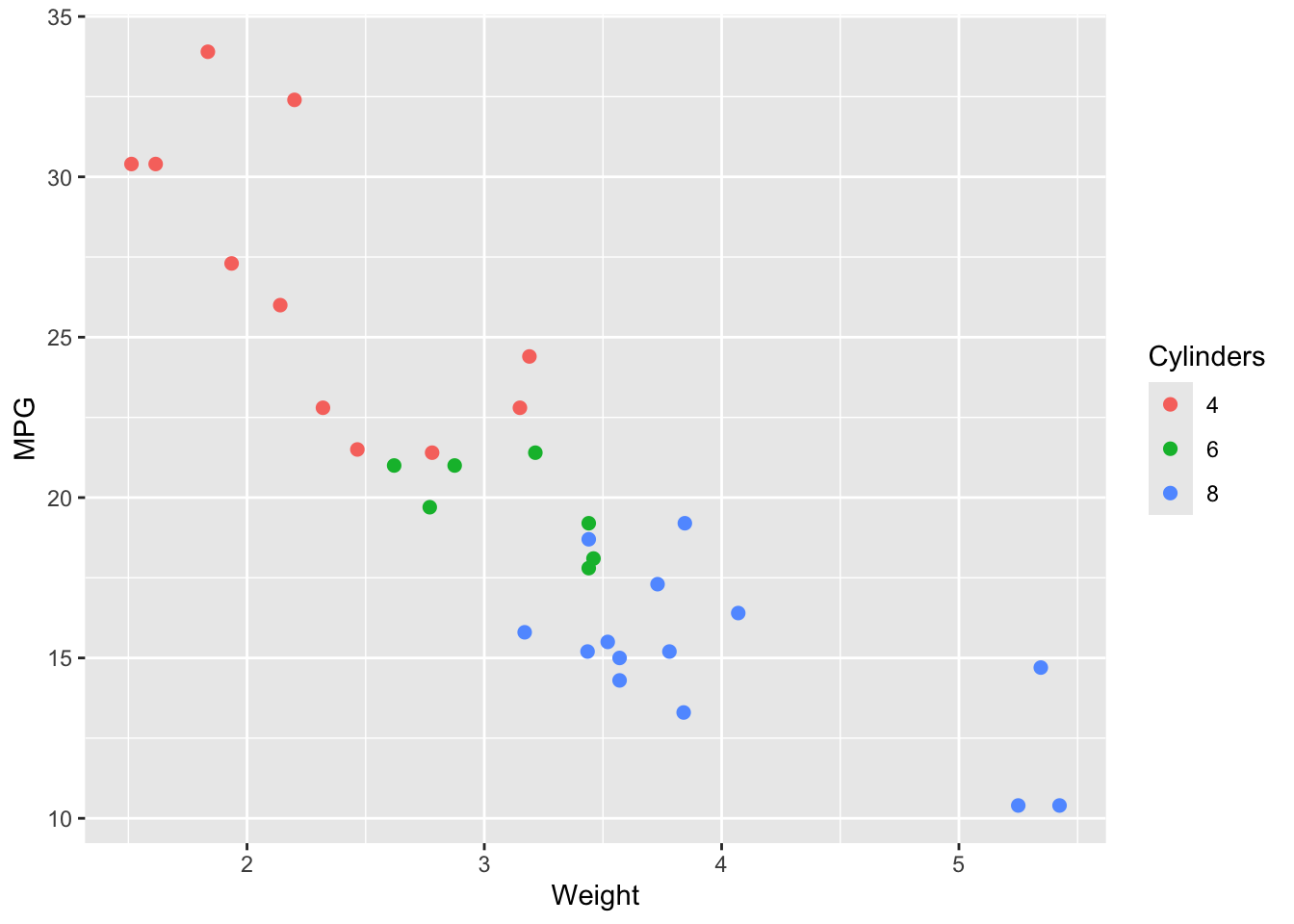

9. Working Directories and Projects

  • Use RStudio Projects and here::here() for reliable paths.
getwd()
[1] "/Users/jihong/Documents/website-jihong/teaching/2024-07-21-applied-multivariate-statistics-esrm64503/Lecture01"
here::here()
[1] "/Users/jihong/Documents/website-jihong"
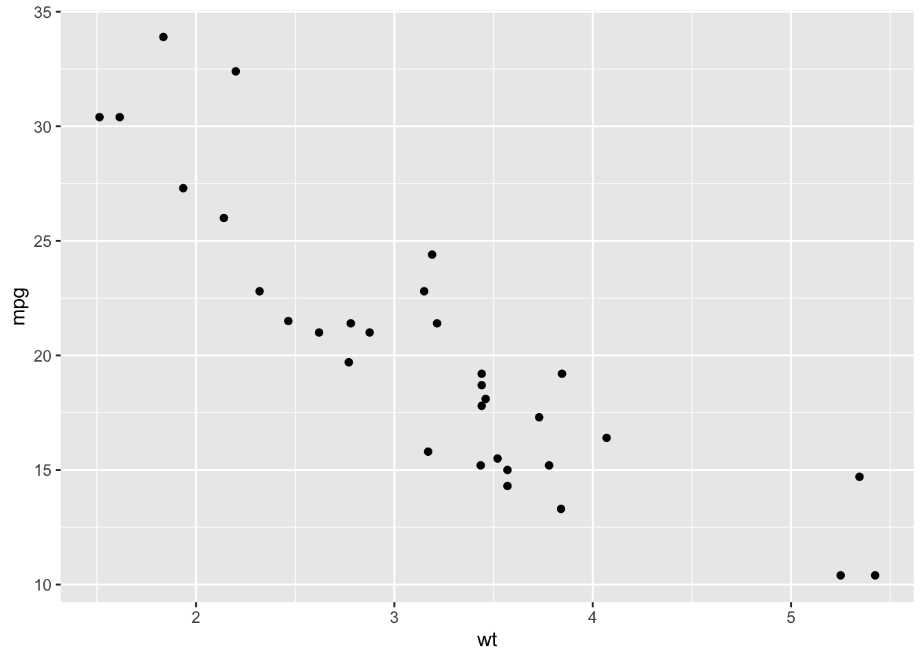
10. Quarto Basics (YAML, Chunks, Render)

  • YAML header controls title, author, format.
  • Chunk options customize behavior (e.g., hide code, set figure captions).
Figure 1: Scatterplot of wt vs mpg
  • Render via the Render button in RStudio or run quarto render in a terminal.

11. Reproducibility

  • Record your session details for reproducibility.
sessionInfo()
R version 4.4.3 (2025-02-28)
Platform: aarch64-apple-darwin20
Running under: macOS Sequoia 15.6

Matrix products: default
BLAS:   /Library/Frameworks/R.framework/Versions/4.4-arm64/Resources/lib/libRblas.0.dylib 
LAPACK: /Library/Frameworks/R.framework/Versions/4.4-arm64/Resources/lib/libRlapack.dylib;  LAPACK version 3.12.0

locale:
[1] en_US.UTF-8/en_US.UTF-8/en_US.UTF-8/C/en_US.UTF-8/en_US.UTF-8

time zone: America/Chicago
tzcode source: internal

attached base packages:
[1] stats     graphics  grDevices utils     datasets  methods   base     

other attached packages:
 [1] here_1.0.1          lubridate_1.9.4     forcats_1.0.0      
 [4] stringr_1.5.1       dplyr_1.1.4         purrr_1.0.4        
 [7] readr_2.1.5         tidyr_1.3.1         tibble_3.2.1       
[10] ggplot2_3.5.2       tidyverse_2.0.0     cmdstanr_0.8.1.9000
[13] rstan_2.32.7        StanHeaders_2.32.10

loaded via a namespace (and not attached):
 [1] gtable_0.3.6         tensorA_0.36.2.1     xfun_0.52           
 [4] QuickJSR_1.7.0       htmlwidgets_1.6.4    processx_3.8.6      
 [7] inline_0.3.21        tzdb_0.5.0           vctrs_0.6.5         
[10] tools_4.4.3          ps_1.9.0             generics_0.1.3      
[13] stats4_4.4.3         curl_6.4.0           parallel_4.4.3      
[16] pkgconfig_2.0.3      checkmate_2.3.2      distributional_0.5.0
[19] RcppParallel_5.1.10  lifecycle_1.0.4      farver_2.1.2        
[22] compiler_4.4.3       munsell_0.5.1        codetools_0.2-20    
[25] htmltools_0.5.8.1    yaml_2.3.10          pillar_1.10.2       
[28] abind_1.4-8          posterior_1.6.1      tidyselect_1.2.1    
[31] digest_0.6.37        stringi_1.8.7        labeling_0.4.3      
[34] rprojroot_2.0.4      fastmap_1.2.0        grid_4.4.3          
[37] colorspace_2.1-1     cli_3.6.5            magrittr_2.0.3      
[40] loo_2.8.0            pkgbuild_1.4.7       withr_3.0.2         
[43] scales_1.3.0         backports_1.5.0      timechange_0.3.0    
[46] rmarkdown_2.29       matrixStats_1.5.0    gridExtra_2.3       
[49] hms_1.1.3            evaluate_1.0.3       knitr_1.50          
[52] V8_6.0.3             rlang_1.1.6          Rcpp_1.0.14         
[55] glue_1.8.0           jsonlite_2.0.0       R6_2.6.1            

12. Getting Help

?mean
help("mean")
example(mean)

mean> x <- c(0:10, 50)

mean> xm <- mean(x)

mean> c(xm, mean(x, trim = 0.10))
[1] 8.75 5.50

13. Next Steps

  • Explore the tidyverse (readr, dplyr, tidyr, ggplot2)
  • Learn Quarto for documents, slides, and websites
  • Practice by importing a dataset, cleaning it, summarizing, and plotting
Back to top