Lecture 13: Mixed ANCOVA

Overview of Lecture 13

1. What is Mixed ANCOVA?
2. Why use Mixed ANCOVA?
3. How to use Mixed ANCOVA (assumptions, hypothesis setup)?
4. Potential issues of using Mixed ANCOVA.

1 Introduction

1.1 Recall: Repeated Measurement ANOVA

1.1.0.1 1-way ANOVA

Student	No Tutor	Once per Week	Daily
Sally
Bob
Martes
…	…	…	…
Omar

• With factorial ANOVA, we put each student in only one condition.
• Then, we look at their grades at the end of the intervention.

1.1.0.2 RM ANOVA

Student	No Tutor	Once per Week	Daily
Sally
Bob
Martes	…	…	…
…	…	…	…
Omar

• With repeated measures ANOVA, we put each student in each of the three conditions.
• Then, we look at their grades at the end of each intervention.
• OR, we can think of following students over time: baseline, 6-weeks into the intervention, follow-up.

1.2 Sphericity check of RM ANOVA

• Check Sphericity!

1.3 RM ANOVA Table

• Repeated Measure ANOVA

1.4 Mixed ANOVA

➤ Recall: Example #1 of repeated measure ANOVA - [Example #1] - Researchers are interested in the effect of drug on blood concentration of histamine at 0, 1, 3, and 5 minutes after injection of the drug. - DV: blood concentration of histamine - Within-subject factor: time (4 levels: 0, 1, 3, and 5 minutes)

• Six dogs, four time points

• Now we want to know if the changes in histamine concentration over time are impacted by drug type

  • Adding a between-subjects variable
  • Dogs in each group receive either carprofen (Novox or Rimadyl), deracoxib (Deramaxx), firocoxib (Previcox), and meloxicam (Metacam) as a treatment for arthritis.
  • Between-subject factor: drug (4 levels)

• We are interested primarily in the interaction of drug and time. ➔ “Mixed” ANOVA!

2 Example of Mixed ANOVA

2.1 Data overview

• First, let’s check if the two measures change over time
  • → Unconditional because no between-subjects factor
  • Significant impact of measure; and significant impact of time.
  • → there are significant differences in two outcomes and three time points.

# Create the data frame
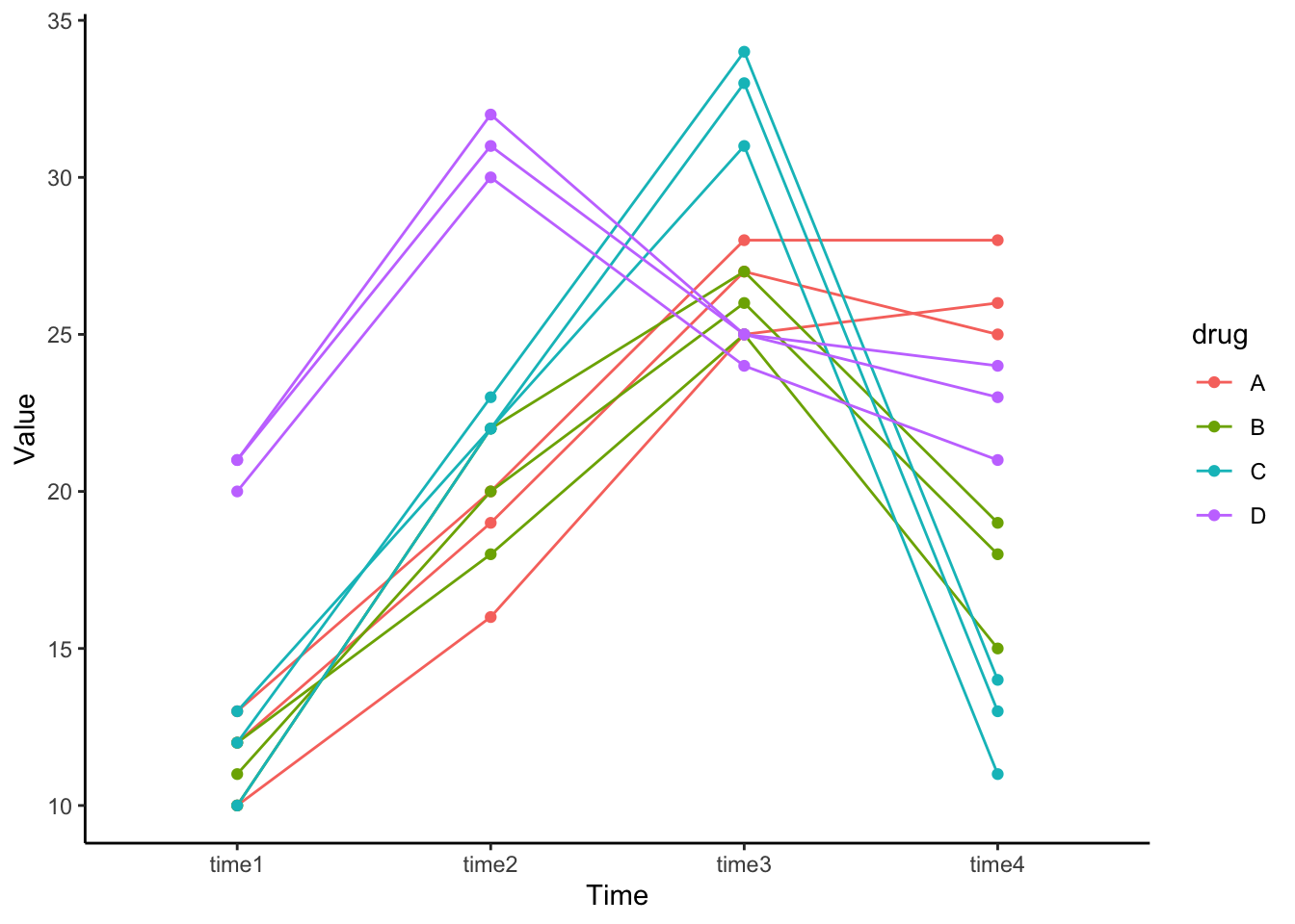
df <- data.frame(
  dog = 1:12,
  time1 = c(10, 12, 13, 12, 11, 10, 10, 12, 13, 20, 21, 21),
  time2 = c(16, 19, 20, 18, 20, 22, 22, 23, 22, 30, 31, 32),
  time3 = c(25, 27, 28, 25, 26, 27, 31, 34, 33, 24, 25, 25),
  time4 = c(26, 25, 28, 15, 18, 19, 11, 14, 13, 21, 24, 23),
  drug = c("A", "A", "A", "B", "B", "B", "C", "C", "C", "D", "D", "D")
)

# View the data frame
df

   dog time1 time2 time3 time4 drug
1    1    10    16    25    26    A
2    2    12    19    27    25    A
3    3    13    20    28    28    A
4    4    12    18    25    15    B
5    5    11    20    26    18    B
6    6    10    22    27    19    B
7    7    10    22    31    11    C
8    8    12    23    34    14    C
9    9    13    22    33    13    C
10  10    20    30    24    21    D
11  11    21    31    25    24    D
12  12    21    32    25    23    D

• We know there is a significant interaction between time and drug

  • We can examine drug differences at each time point!

library(tidyverse)
df |> 
  pivot_longer(starts_with("time"), names_to = "Time", values_to = "Value") |> 
  mutate(Time = factor(Time, levels = paste0("time", 1:4))) |> 
  ggplot(aes(x = Time, y = Value, color = drug, group = dog)) +
  geom_path() +
  geom_point() +
  theme_classic()

Below is a full formal, academic-style write-up and corresponding R code for conducting a mixed ANOVA on the dataset you provided:

---

2.1.1 Study Setup

Outcome Variable:
- Dog performance scores at four different times: time1, time2, time3, and time4.

Independent Variables (IVs):
- Within-Subjects IV: Time (four repeated measures: time1, time2, time3, time4)
- Between-Subjects IV: Drug (four levels: A, B, C, D)

Research Question:
- Main Effects:
- Does time influence the dog’s performance?
- Does the drug type influence the dog’s performance? - Interaction Effect:
- Does the effect of time on performance differ depending on drug type?

---

2.1.2 R Code: Data Preparation and Mixed ANOVA

# Load necessary libraries
library(tidyverse)
library(ez)

# Reshape the data from wide to long format
df_long <- df %>%
  pivot_longer(
    cols = time1:time4,
    names_to = "time",
    values_to = "performance"
  )

# Ensure factors are properly coded
df_long$dog <- factor(df_long$dog)
df_long$time <- factor(df_long$time, levels = c("time1", "time2", "time3", "time4"))
df_long$drug <- factor(df_long$drug)

# Perform the mixed ANOVA
anova_result <- ezANOVA(
  data = df_long,
  dv = performance,
  wid = dog,
  within = time,
  between = drug,
  type = 3,
  detailed = TRUE
)

# Print ANOVA results
print(anova_result)

$ANOVA
       Effect DFn DFd        SSn      SSd          F            p p<.05
1 (Intercept)   1   8 21126.0208 43.33333 3900.18846 4.804763e-12     *
2        drug   3   8   255.8958 43.33333   15.74744 1.017647e-03     *
3        time   3  24  1200.5625 22.66667  423.72794 6.547316e-21     *
4   drug:time   9  24   658.5208 22.66667   77.47304 1.538964e-15     *
        ges
1 0.9968856
2 0.7949647
3 0.9478905
4 0.9089053

$`Mauchly's Test for Sphericity`
     Effect         W          p p<.05
3      time 0.1921751 0.05196908      
4 drug:time 0.1921751 0.05196908      

$`Sphericity Corrections`
     Effect       GGe        p[GG] p[GG]<.05       HFe        p[HF] p[HF]<.05
3      time 0.6306601 6.734691e-14         * 0.8201143 1.687143e-17         *
4 drug:time 0.6306601 2.018604e-10         * 0.8201143 4.729484e-13         *

---

2.1.3 Assumption Checking

2.1.3.1 Sphericity (for within-subjects factor Time)

# Mauchly’s Test for Sphericity is included in ezANOVA output
anova_result$`Mauchly's Test for Sphericity`

     Effect         W          p p<.05
3      time 0.1921751 0.05196908      
4 drug:time 0.1921751 0.05196908      

• If p < .05, sphericity is violated, and corrections (Greenhouse-Geisser or Huynh-Feldt) must be applied.

---

2.1.4 Results

Suppose the output from ezANOVA indicates the following hypothetical results (you would replace with actual output):

anova_result$ANOVA

       Effect DFn DFd        SSn      SSd          F            p p<.05
1 (Intercept)   1   8 21126.0208 43.33333 3900.18846 4.804763e-12     *
2        drug   3   8   255.8958 43.33333   15.74744 1.017647e-03     *
3        time   3  24  1200.5625 22.66667  423.72794 6.547316e-21     *
4   drug:time   9  24   658.5208 22.66667   77.47304 1.538964e-15     *
        ges
1 0.9968856
2 0.7949647
3 0.9478905
4 0.9089053

---

2.1.5 Interpretation

• Main Effect of Time:
  There is a significant effect of time on dog performance, ( F(3, 24) = 423.72, p < .001, _p^2 = 0.94 ). Dogs’ scores changed significantly across the four time points.

• Main Effect of Drug:
  There is a significant main effect of drug, ( F(3, 8) = 15.74, p < .001, _p^2 = 0.79 ). Dogs receiving different drug treatments showed different overall levels of performance.

• Interaction between Time and Drug:
  A significant interaction between time and drug was found, ( F(9, 24) = 77.47, p < .001, _p^2 = 0.90 ), suggesting that the pattern of change over time differed depending on the drug administered.

---

2.1.6 Post-Hoc and Follow-Up Analyses

• Given significant interaction, post-hoc comparisons would be necessary to explore:

  • Which time points differ within each drug.
  • How the drugs differ at each time point.

This can be done using pairwise comparisons with Bonferroni correction.

Example in R:

# Post-hoc analysis
library(emmeans)

model2 <- aov(performance ~ drug * time + Error(dog/time), data = df_long)
emmeans(model2, pairwise ~ drug | time, adjust = "bonferroni")

$emmeans
time = time1:
 drug emmean    SE df lower.CL upper.CL
 A      11.7 0.829 17     9.92     13.4
 B      11.0 0.829 17     9.25     12.7
 C      11.7 0.829 17     9.92     13.4
 D      20.7 0.829 17    18.92     22.4

time = time2:
 drug emmean    SE df lower.CL upper.CL
 A      18.3 0.829 17    16.58     20.1
 B      20.0 0.829 17    18.25     21.7
 C      22.3 0.829 17    20.58     24.1
 D      31.0 0.829 17    29.25     32.7

time = time3:
 drug emmean    SE df lower.CL upper.CL
 A      26.7 0.829 17    24.92     28.4
 B      26.0 0.829 17    24.25     27.7
 C      32.7 0.829 17    30.92     34.4
 D      24.7 0.829 17    22.92     26.4

time = time4:
 drug emmean    SE df lower.CL upper.CL
 A      26.3 0.829 17    24.58     28.1
 B      17.3 0.829 17    15.58     19.1
 C      12.7 0.829 17    10.92     14.4
 D      22.7 0.829 17    20.92     24.4

Warning: EMMs are biased unless design is perfectly balanced 
Confidence level used: 0.95 

$contrasts
time = time1:
 contrast estimate   SE df t.ratio p.value
 A - B       0.667 1.17 17   0.569  1.0000
 A - C       0.000 1.17 17   0.000  1.0000
 A - D      -9.000 1.17 17  -7.675  <.0001
 B - C      -0.667 1.17 17  -0.569  1.0000
 B - D      -9.667 1.17 17  -8.244  <.0001
 C - D      -9.000 1.17 17  -7.675  <.0001

time = time2:
 contrast estimate   SE df t.ratio p.value
 A - B      -1.667 1.17 17  -1.421  1.0000
 A - C      -4.000 1.17 17  -3.411  0.0199
 A - D     -12.667 1.17 17 -10.802  <.0001
 B - C      -2.333 1.17 17  -1.990  0.3776
 B - D     -11.000 1.17 17  -9.381  <.0001
 C - D      -8.667 1.17 17  -7.391  <.0001

time = time3:
 contrast estimate   SE df t.ratio p.value
 A - B       0.667 1.17 17   0.569  1.0000
 A - C      -6.000 1.17 17  -5.117  0.0005
 A - D       2.000 1.17 17   1.706  0.6377
 B - C      -6.667 1.17 17  -5.685  0.0002
 B - D       1.333 1.17 17   1.137  1.0000
 C - D       8.000 1.17 17   6.822  <.0001

time = time4:
 contrast estimate   SE df t.ratio p.value
 A - B       9.000 1.17 17   7.675  <.0001
 A - C      13.667 1.17 17  11.655  <.0001
 A - D       3.667 1.17 17   3.127  0.0368
 B - C       4.667 1.17 17   3.980  0.0058
 B - D      -5.333 1.17 17  -4.548  0.0017
 C - D     -10.000 1.17 17  -8.528  <.0001

P value adjustment: bonferroni method for 6 tests 

emmeans(model2, pairwise ~ time | drug, adjust = "bonferroni")

$emmeans
drug = A:
 time  emmean    SE df lower.CL upper.CL
 time1   11.7 0.829 17     9.92     13.4
 time2   18.3 0.829 17    16.58     20.1
 time3   26.7 0.829 17    24.92     28.4
 time4   26.3 0.829 17    24.58     28.1

drug = B:
 time  emmean    SE df lower.CL upper.CL
 time1   11.0 0.829 17     9.25     12.7
 time2   20.0 0.829 17    18.25     21.7
 time3   26.0 0.829 17    24.25     27.7
 time4   17.3 0.829 17    15.58     19.1

drug = C:
 time  emmean    SE df lower.CL upper.CL
 time1   11.7 0.829 17     9.92     13.4
 time2   22.3 0.829 17    20.58     24.1
 time3   32.7 0.829 17    30.92     34.4
 time4   12.7 0.829 17    10.92     14.4

drug = D:
 time  emmean    SE df lower.CL upper.CL
 time1   20.7 0.829 17    18.92     22.4
 time2   31.0 0.829 17    29.25     32.7
 time3   24.7 0.829 17    22.92     26.4
 time4   22.7 0.829 17    20.92     24.4

Warning: EMMs are biased unless design is perfectly balanced 
Confidence level used: 0.95 

$contrasts
drug = A:
 contrast      estimate    SE df t.ratio p.value
 time1 - time2   -6.667 0.793 24  -8.402  <.0001
 time1 - time3  -15.000 0.793 24 -18.904  <.0001
 time1 - time4  -14.667 0.793 24 -18.484  <.0001
 time2 - time3   -8.333 0.793 24 -10.502  <.0001
 time2 - time4   -8.000 0.793 24 -10.082  <.0001
 time3 - time4    0.333 0.793 24   0.420  1.0000

drug = B:
 contrast      estimate    SE df t.ratio p.value
 time1 - time2   -9.000 0.793 24 -11.342  <.0001
 time1 - time3  -15.000 0.793 24 -18.904  <.0001
 time1 - time4   -6.333 0.793 24  -7.982  <.0001
 time2 - time3   -6.000 0.793 24  -7.562  <.0001
 time2 - time4    2.667 0.793 24   3.361  0.0156
 time3 - time4    8.667 0.793 24  10.922  <.0001

drug = C:
 contrast      estimate    SE df t.ratio p.value
 time1 - time2  -10.667 0.793 24 -13.443  <.0001
 time1 - time3  -21.000 0.793 24 -26.465  <.0001
 time1 - time4   -1.000 0.793 24  -1.260  1.0000
 time2 - time3  -10.333 0.793 24 -13.023  <.0001
 time2 - time4    9.667 0.793 24  12.182  <.0001
 time3 - time4   20.000 0.793 24  25.205  <.0001

drug = D:
 contrast      estimate    SE df t.ratio p.value
 time1 - time2  -10.333 0.793 24 -13.023  <.0001
 time1 - time3   -4.000 0.793 24  -5.041  0.0002
 time1 - time4   -2.000 0.793 24  -2.521  0.1127
 time2 - time3    6.333 0.793 24   7.982  <.0001
 time2 - time4    8.333 0.793 24  10.502  <.0001
 time3 - time4    2.000 0.793 24   2.521  0.1127

P value adjustment: bonferroni method for 6 tests 

---

2.1.7 Visualization of Interaction

To better understand the interaction effect, an interaction plot is highly recommended:

# Interaction Plot
library(ggplot2)

ggplot(df_long, aes(x = time, y = performance, group = drug, color = drug)) +
  stat_summary(fun = mean, geom = "line") +
  stat_summary(fun = mean, geom = "point") +
  labs(
    title = "Dog Performance Across Time by Drug Type",
    x = "Time",
    y = "Mean Performance"
  ) +
  theme_minimal()

2.1.8 Summary

Aspect	Summary
Outcome	Dog performance scores at four time points
Within-Subjects IV	Time (4 levels: time1 to time4)
Between-Subjects IV	Drug (4 levels: A, B, C, D)
Main Effects	Significant for both Time and Drug
Interaction Effect	Significant Time × Drug Interaction
Assumptions	Normality and Sphericity were assessed
Post-Hoc Analysis	Recommended for interpreting interaction effects
Visualization	Interaction plot recommended

3 Issues of Mixed ANOVA

3.1 Potential probelms to be considered

1. Missing Data on the Outcome

• One of the biggest problems with traditional repeated measures ANOVA is missing data on the response variable.

• The problem is that repeated measures ANOVA treats each measurement as a separate variable.

• RMANOVA uses listwise deletion: if one measurement is missing, the entire case gets dropped.

2. Unbalanced number of repeats across individuals

• A related problem is imbalance in the number of repeated responses from each individual.

• This is common in observed data, where the number of repeats is uncontrollable.
  You measure a response each time some occurrence happens.

  • Ex: Students using the tutoring lab. Some students come in once/week, others daily, some others come multiple times/day.
  • We measure their satisfaction at each lab session.
  • Problem: I have 10 measurements for some people, 2 for other people, etc.

• This causes two problems:

  • Different number of response variables for each individual. If some have missing data in the last few responses, they’ll get dropped. (That dropping/deletion problem again! Ugh!)
  • ANOVA will compare the responses to each other, assuming that each one represents a different condition (time point).
    There is no way to turn off that comparison.

• In clinical trials, even though there may be a planned number of repeated measurements, participants don’t always come back:

  • They may not be seeing results and give up
  • They may pass away or be too sick to return
  • Participation may be too burdensome

➤ Survival analysis is one approach to handling this type of censored data.

3. When time is continuous

• In some studies, the amount of time that has passed between repeated measurements is important.
  • ➤ In other words, you want to treat the within-subjects effect of time as a continuous, quantitative variable.
  • ➤ Ex: After each mile someone runs in a half-marathon, you take their pulse.
  • ➤ There will be 14-time measurements (including baseline).
  • ➤ But not everyone runs the miles at the same pace
    • Some will take 8 minutes, some 11, others 6.45 minutes, etc.
    • So, time between measurements matters, and is continuous.
• Repeated measures ANOVA can only account for categorical repeated measurements (e.g., after mile 1, mile 2, etc.).

4. Time-varying covariates

• In some studies, important predictor variables are measured on each repeat, right along with the response.
  • [ex.] Weight and wingspan may be measured as predictors of athlete endurance, but weight changes at each measurement
    (it is not held constant throughout the experiment), whereas wingspan probably will not change over the course of the experiment.
• RMANOVA assumes our covariates are the same the entire time.

5. Three (or more) level models

• If the subjects themselves are not only measured multiple times, but also clustered into some other groups, you have a three-level model.

  • For example, you may have students measured over time, but students are also clustered within classrooms.
  • Patients measured over time are also clustered into medical centers.

• In all these cases, the repeated measures ANOVA can account for the repeats over time, but not the clustering.

• Multilevel or hierarchical models are other names for mixed models.

  • We offer a course in this: ESRM 6513. Hierarchical Linear Modeling. 3 Hours.
  • This course covers the theory and applications of hierarchical linear modeling (HLM), also known as multilevel modeling.
    Both the conceptual and methodological issues for analyses of nested (clustered) data in using HLM will be reviewed,
    including linear models, non-linear models, growth models, and some alternative designs.
    Prerequisite: ESRM 6413 and ESRM 6423. (Typically offered: Fall Even Years)

6. Repeated measures across people and items

• There is a repeated measures design that occurs in specific experimental studies, common in linguistics and psychology.
  • Each subject is repeatedly measured across many trials.
  • Each trial contains one item, and there are multiple items for each condition. - Ex: Measure of reaction time of 50 participants to each of 20 high-frequency and 20 low-frequency words.
  • 40 reaction times are repeated across each participant.
  • Each word also has 50 repeated measurements (one per participant), and those are also likely to be correlated.
    Some words will elicit faster times than others, even within the same condition.
• Repeated measures ANOVA can only account for the repeat across one type of subject (trials or words, not both).

7. Non-continuous outcomes

• If your outcome is categorical or a count outcome, RMANOVA is not going to work.
  • Neither will a mixed model in this case.
• Luckily, there are other options: logistic regression and Poisson regression are two common approaches for yes/no and count outcomes, respectively.

Fin